Logistic Regression: Definition, Formula and Examples
By Dr. Zubair Khalid, DVM, MS, PhD ·
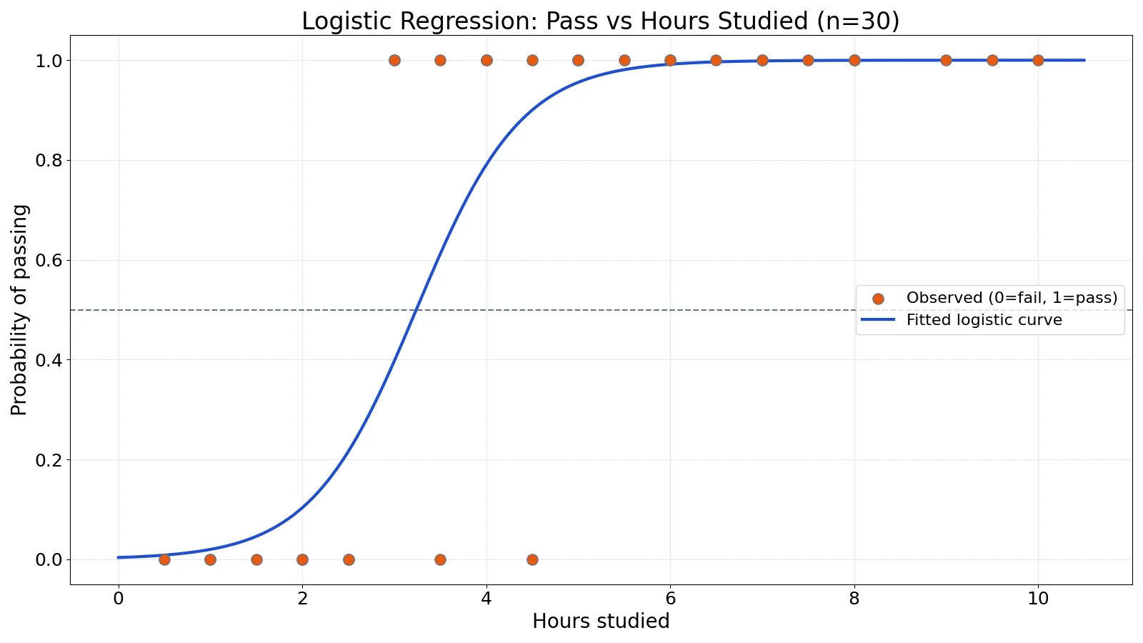
Logistic regression is a statistical method for modeling a binary outcome, such as pass/fail, yes/no, or alive/dead, from one or more predictor variables. Instead of predicting the outcome directly, it estimates the probability that the outcome equals 1. Coefficients are usually converted to odds ratios, which tell you how the odds of the outcome change when a predictor increases by one unit.
Quick Answer
- Logistic regression models the probability of a binary outcome using an S-shaped curve bounded between 0 and 1.
- The model fits a linear equation to the log-odds of the outcome, then converts it back to a probability with the logistic function.
- Coefficients are on the log-odds scale. Exponentiating a coefficient gives an odds ratio.
- An odds ratio above 1 means higher predictor values raise the odds of the event. Below 1 means they lower it.
- It handles both categorical and continuous predictors, which is a key advantage over simple odds ratio calculations [1].
What Is Logistic Regression?
Logistic regression is a statistical method that predicts the probability of a yes/no outcome from one or more predictors. It fits a linear equation to the log-odds of the event, then converts that value into a probability between 0 and 1 using the logistic function. In one sentence: it models how the odds of a binary event change as predictor values change.
The formula has two parts. The logit equation is logit(p) = b0 + b1x1 + ... + bkxk, and the probability is recovered as p = 1 / (1 + e^(-logit)). The coefficients b1 through bk are on the log-odds scale, so exponentiating one gives an odds ratio.
A quick example makes it concrete. Suppose a model of exam pass versus hours studied gives an intercept of -5.65 and a slope of 1.74. A student with 5 hours has a logit of -5.65 + 1.74 × 5 = 3.07, which converts to a predicted pass probability of about 0.96. The slope's odds ratio is e^1.74 = 5.72, meaning each extra hour multiplies the odds of passing by roughly 5.7.
| Question | Short answer |
|---|---|
| What kind of outcome does it model? | A binary outcome coded 0 and 1 |
| What do the coefficients mean? | Change in log-odds per one-unit predictor increase |
| How do I read an odds ratio? | Above 1 raises the odds, below 1 lowers them, 1 means no association |
| Is it the same as linear regression? | No. Linear regression predicts a continuous mean; this predicts log-odds of a binary event |
| Does it need one predictor only? | No. It accepts many predictors, continuous or categorical, and adjusts each for the others |
The analysis is called logistic because of the logistic (S-shaped) curve it uses, and regression because it relates an outcome to predictors. It is a type of generalized linear model with a logit link. The fitted equation is what people mean by the logistic regression model: a set of estimated coefficients plus the link that turns them into probabilities. Fitting means finding the coefficients that make the observed data most likely, which is done by maximum likelihood rather than ordinary least squares.
What Logistic Regression Means
In plain terms, logistic regression answers a probability question: given what we know about a case, how likely is the outcome? If you want to predict whether a student passes an exam based on hours studied, logistic regression gives you a probability for each student, not a hard yes or no.
The precise definition is narrower. Logistic regression is a statistical technique that evaluates the relationship between one or more predictor variables, categorical or continuous, and an outcome that is binary or dichotomous [2]. It is a generalized linear model that uses the logit link function to connect a linear combination of predictors to the probability of the outcome [3].
The method works much like multiple linear regression, with the difference that the response variable is binomial. The result is the impact of each variable on the odds ratio of the event of interest, and the main advantage is that it avoids confounding effects by analyzing all variables together [1].
How It Works
The model has two layers. First, a linear equation produces a value called the logit or log-odds:
$$ \text{logit}(p) = b_0 + b_1 x_1 + b_2 x_2 + \dots + b_k x_k $$
Then the logistic function converts that logit into a probability:
$$ P(y = 1) = \frac{1}{1 + e^{-(b_0 + b_1 x_1 + \dots + b_k x_k)}} $$
Each symbol has a specific role:
| Symbol | Meaning |
|---|---|
| $P(y = 1)$ | Probability that the outcome equals 1 |
| $b_0$ | Intercept, the log-odds when all predictors are 0 |
| $b_1 \dots b_k$ | Coefficients, one per predictor |
| $x_1 \dots x_k$ | Predictor values for a given case |
| $e$ | Euler's number, about 2.718 |
The logit can take any value from negative to positive infinity. The logistic function maps it into the 0 to 1 range, which is what makes the model valid for probabilities. Because the outcome is binary, the model is fit by maximum likelihood, which finds the coefficients that make the observed data most probable. The log-likelihood measures how well the fitted model explains the observed outcomes, and lower (more negative) values indicate a worse fit for the same data.
Worked Example
The dataset contains 30 students, with hours studied and whether each student passed (1) or failed (0).
| Hours | Passed | Hours | Passed | Hours | Passed |
|---|---|---|---|---|---|
| 0.5 | 0 | 1 | 0 | 2.5 | 0 |
| 1 | 0 | 2 | 0 | 3.5 | 1 |
| 1.5 | 0 | 3 | 1 | 4.5 | 1 |
| 2 | 0 | 4 | 1 | 5.5 | 1 |
| 2.5 | 0 | 5 | 1 | 6 | 1 |
| 3 | 1 | 6 | 1 | 7 | 1 |
| 3.5 | 0 | 6.5 | 1 | 8 | 1 |
| 4 | 1 | 7 | 1 | 9 | 1 |
| 4.5 | 0 | 7.5 | 1 | 9.5 | 1 |
| 5 | 1 | 8 | 1 | 10 | 1 |
The model form is:
$$ P(\text{pass}) = \frac{1}{1 + e^{-(b_0 + b_1 \cdot \text{hours})}} $$
Fitting the model gives an intercept of $b_0 = -5.6498$ with a standard error of 2.4294 and a p-value of 0.0200. The slope is $b_1 = 1.7442$ with a standard error of 0.7122 and a p-value of 0.0143. The log-likelihood is $-7.0975$.
The odds ratio for hours is $e^{1.7442} = 5.7212$, with a 95% confidence interval of [1.4168, 23.1033]. Because the interval excludes 1, the effect is statistically significant at the 5% level.
To predict a student who studied 5 hours, plug the values into the logit:
$$ \text{logit} = -5.6498 + 1.7442 \times 5.0 = 3.0711 $$
The odds are $e^{3.0711} = 21.5657$, and the probability is:
$$ p = \frac{1}{1 + e^{-3.0711}} = 0.9557 $$
So a student with 5 hours of study has an estimated 95.57% chance of passing.
Here is the Python code that produces these estimates:
import statsmodels.api as sm
X = sm.add_constant(df['hours'])
model = sm.Logit(df['passed'], X).fit()
print(model.params)
print(model.conf_int())
Output:
const = -5.6498, hours = 1.7442; odds ratio = 5.7212 (95% CI 1.4168 to 23.1033); P(pass | 5h) = 0.9557How to Interpret It
The slope of 1.7442 is on the log-odds scale, which is hard to read directly. Exponentiating it gives the odds ratio of 5.7212. The interpretation is that each additional hour of study multiplies the odds of passing by about 5.72. This is a multiplicative effect on odds, not on probability.
The intercept of -5.6498 is the log-odds of passing when hours equals 0. Its odds ratio is $e^{-5.6498} = 0.0035$, which is the baseline odds for a student who did not study.
Predicted probabilities are often more intuitive than odds ratios. At 5 hours the model predicts a 0.9557 probability of passing. At 2 hours the logit is $-5.6498 + 1.7442 \times 2 = -2.1614$, giving a probability of 0.1032. The curve rises steeply in the middle and flattens at both ends.
When you have several predictors, each odds ratio is adjusted for the others in the model. That adjustment is what controls for confounding [1]. If you are new to the idea of a predictor variable, the definition and examples of an explanatory variable cover the terminology.
When to Use It (and when not to)
Use logistic regression when the outcome has exactly two categories and you want to model the probability of one of them. It suits both experimental and observational data, and it accepts a mix of continuous and categorical predictors [2]. It is standard in clinical research for outcomes like death, infection, or response to treatment [1].
Do not use it when the outcome is continuous. Linear regression is the right tool there, and the assumptions of linear regression differ in important ways. Do not use it when the outcome has three or more unordered categories, since that requires multinomial logistic regression. For ordered categories, ordinal logistic regression is the appropriate extension.
Sample size matters. With few events per predictor, estimates become unstable and confidence intervals grow very wide. A common rule of thumb is at least 10 events per predictor variable, though this is a guideline and not a hard cutoff [2].
Logistic Regression vs Linear Regression
Both methods fit a linear combination of predictors, but they differ in what they model and what the coefficients mean.
| Feature | Logistic Regression | Linear Regression |
|---|---|---|
| Outcome type | Binary (0/1) | Continuous |
| What is modeled | Log-odds of the outcome | Mean of the outcome |
| Link function | Logit | Identity |
| Coefficient scale | Log-odds | Outcome units |
| Typical effect measure | Odds ratio | Change in mean |
| Fitting method | Maximum likelihood | Ordinary least squares |
| Predicted values | Probabilities between 0 and 1 | Any real number |
The key practical difference is that a linear regression can predict values outside the possible range of a binary outcome, while logistic regression cannot. If you want a broader grounding in the family of methods, see this practical introduction to regression analysis.
Common Mistakes
- Reading coefficients as probability changes. A coefficient of 1.7442 does not mean the probability rises by 1.7442. Exponentiate it to get the odds ratio, then convert to probabilities at specific predictor values if you need them.
- Ignoring the confidence interval on the odds ratio. An odds ratio of 5.72 sounds large, but the interval here runs from 1.42 to 23.10. Report the interval, not just the point estimate.
- Treating the odds ratio as a risk ratio. Odds ratios overstate risk ratios when the outcome is common. For frequent outcomes, the two diverge substantially.
- Dropping predictors because a p-value is above 0.05. A predictor can matter for adjustment even when it is not significant on its own. Removing it can bias the other estimates.
- Using accuracy alone to judge the model. With imbalanced outcomes, a model that always predicts the majority class can score high accuracy while being useless. Look at the confusion matrix and other metrics [4].
- Forgetting to check the linearity of the logit. Logistic regression assumes the log-odds change linearly with each continuous predictor. A curved relationship needs a transformation or a spline term [3].
Limitations
Logistic regression cannot capture complex interactions unless you specify them by hand. It also assumes independent observations, so clustered data such as students within classrooms need a different approach [5]. Complete separation, where a predictor perfectly splits the outcome, can push coefficients toward infinity and make standard errors unreliable.
The model gives you probabilities and odds ratios, not causal effects. A large odds ratio from observational data can reflect confounding by variables you did not measure. Diagnostics for logistic regression differ from those for ordinary least squares, and residual checks follow their own logic [5]. If you want to understand how the fit is judged, the definition and formula for log-likelihood explains the quantity being maximized.
The Logistic Regression Equation, Step by Step
The equation looks intimidating but is just two short steps. Step one builds a score from the predictors. Step two squeezes that score into a probability.
Step one, the linear score. Add the intercept to each predictor multiplied by its coefficient: z = b0 + b1x1 + b2x2 + ... This z is the log-odds, also called the logit. It can be any real number, positive or negative.
Step two, the conversion. Apply p = 1 / (1 + e^(-z)). Large positive z gives p near 1. Large negative z gives p near 0. A z of 0 gives p of exactly 0.5.
Reading it backward. If you know a probability, the log-odds is ln(p / (1 - p)). A probability of 0.5 has log-odds 0. A probability of 0.9 has log-odds ln(9) = 2.20. A probability of 0.1 has log-odds ln(1/9) = -2.20. This symmetry is why the logit scale is convenient: equal distances above and below zero mean equal swings in odds.
Why not fit a straight line to the 0/1 outcome? A straight line can predict values below 0 or above 1, which are impossible probabilities. The S-curve stays inside the valid range and matches the way real binary data behave: flat at the extremes, steep in the middle.
What the fit operation produces
When software fits the model, it reports a coefficient for every term plus an intercept, each with a standard error and a p-value, and an overall log-likelihood. The fitted equation is simply those numbers placed into the logit formula. In the student example the fit yields logit(p) = -5.6498 + 1.7442 × hours. That single line is the whole model. Everything else, odds ratios and predicted probabilities, is derived from it.
Odds, Risk and the Odds Ratio Trap
Odds and probability are different quantities, and mixing them is the most common source of confusion.
| Quantity | Formula | Example when p = 0.8 |
|---|---|---|
| Probability | p | 0.80 |
| Odds | p / (1 - p) | 4.0 |
| Log-odds | ln(odds) | 1.386 |
An odds ratio compares odds between two groups or two predictor values. If the odds of passing are 4.0 at 6 hours and 1.0 at 5 hours, the odds ratio is 4.0. The corresponding probabilities might be 0.80 and 0.50, a risk ratio of 1.6. The odds ratio of 4.0 is far from the risk ratio of 1.6.
This gap grows as the outcome becomes more common. When the event is rare, the odds ratio is close to the risk ratio and can be read loosely as a relative risk. When the event is common, the odds ratio overstates the relative change in risk. A clinician reading an odds ratio of 3 for a frequent outcome should not conclude that risk triples. This is why reporting predicted probabilities alongside odds ratios is good practice.
A second worked example with two predictors
Imagine predicting whether a patient is readmitted within 30 days, using age and a comorbidity count. Suppose the fitted equation is logit(p) = -3.2 + 0.03 × age + 0.6 × comorbidities. For a 70-year-old with 2 comorbidities, z = -3.2 + 2.1 + 1.2 = 0.1, giving p = 1 / (1 + e^(-0.1)) = 0.525. The odds ratio for each comorbidity is e^0.6 = 1.82, adjusted for age. The odds ratio for each year of age is e^0.03 = 1.03, adjusted for comorbidities. Note that the age effect looks tiny per year but compounds over decades.
Common Misconceptions About Logistic Regression
"The coefficient is the change in probability." No. The coefficient is a change in log-odds. Probability change depends on where you start on the curve, because the S-shape is steep in the middle and flat at the ends. The same coefficient produces a bigger probability shift near p = 0.5 than near p = 0.05.
"A high odds ratio proves causation." No. Observational data can produce large odds ratios from confounding alone. The model adjusts for measured variables but cannot adjust for what was never recorded.
"The model predicts a category." The raw model outputs a probability. Turning it into a yes/no decision requires a cutoff, and the choice of cutoff is a separate judgment based on the cost of false positives versus false negatives.
"Accuracy tells you if the model is good." With a rare outcome, predicting "no" for everyone can score high accuracy while catching zero events. Discrimination measures such as the area under the ROC curve, and calibration checks comparing predicted with observed rates, are more informative [4].
"More predictors always improve it." Adding predictors can overfit, especially with few events. Each added term needs enough outcome events to estimate it stably [2].
"Separation just means a strong effect." When a predictor perfectly separates the two outcome groups, the likelihood keeps rising as the coefficient grows, so estimates can diverge and standard errors become unreliable. This is a fitting problem, not evidence of a perfect predictor.
Checking Whether the Model Fits
Fitting coefficients is only half the job. A usable model also needs to be checked.
Linearity of the logit. For each continuous predictor, the log-odds should change roughly linearly. A curved pattern suggests a transformation or a spline term [3].
Calibration. Group cases by predicted probability and compare the average prediction with the observed event rate in each group. A model that predicts 0.30 on average for a group where 30 percent actually have the event is well calibrated.
Discrimination. How well does the model rank cases? A model that gives higher probabilities to those who have the event is discriminating well, even if its absolute probabilities are off.
Influence and outliers. A few unusual cases can pull coefficients. Check whether removing a handful of points changes the conclusions.
Independence. Standard errors assume observations are independent. Clustered data, such as patients within hospitals, need methods that account for the grouping [5].
Frequently Asked Questions
What is the difference between logistic regression and linear regression?
Linear regression predicts a continuous outcome and models its mean. Logistic regression predicts a binary outcome and models the log-odds of the event. The coefficients in linear regression are changes in the outcome, while coefficients in logistic regression are changes in log-odds that convert to odds ratios.
How do I interpret an odds ratio in logistic regression?
An odds ratio of 5.72 for hours studied means each extra hour multiplies the odds of passing by 5.72. An odds ratio of 1 means no association. Values below 1 mean the predictor lowers the odds. Always report the confidence interval alongside the point estimate.
Can logistic regression handle more than one predictor?
Yes. Adding predictors extends the logit equation with one term per predictor. Each odds ratio is then adjusted for the other variables in the model, which reduces confounding [1]. This is the main reason logistic regression is preferred over calculating a single crude odds ratio.
What sample size do I need for logistic regression?
There is no single number. A common guideline is at least 10 events in the smaller outcome category per predictor variable [2]. With rare outcomes or many predictors, estimates become unstable. Simulation or exact methods may be needed for small samples.
What does the intercept mean in logistic regression?
The intercept is the log-odds of the outcome when every predictor equals 0. In the worked example, the intercept of -5.6498 gives a baseline odds of 0.0035 for a student with 0 hours of study. The intercept is often not meaningful on its own when 0 is outside the realistic range of the predictors.
References
- Understanding logistic regression analysis - PMC
- Ranganathan P, Pramesh CS, Aggarwal R. (2017). Common pitfalls in statistical analysis: Logistic regression. Perspectives in clinical research
- 8.4: Introduction to Logistic Regression - Statistics LibreTexts./08%3A_Multiple_and_Logistic_Regression/8.04%3A_Introduction_to_Logistic_Regression)
- 3.4. Metrics and scoring: quantifying the quality of predictions, scikit-learn 1.9.1 documentation
- Logistic Regression | Stata Data Analysis Examples
Further Reading
Related Articles
- Explanatory Variable: Definition, Examples and Role in Regression
- What Is Log-Likelihood? Definition, Formula and Examples
- Bivariate Data: Definition, Examples and Analysis
- Multivariate Analysis: Definition, Methods and Examples
- Quadratic Regression Analysis: Equation and Example
- Logistic Regression in Clinical Research
- What is Regression Analysis? A Practical Introduction
- Regression Analysis Biostatistics