Quadratic Regression Analysis: Equation and Example

By Dr. Zubair Khalid, DVM, MS, PhD · 2026-10-03

Quadratic regression analysis fits an equation with a squared term so a curved relationship between two variables can be modeled. Instead of a straight line, you estimate a parabola of best fit. This article shows the equation, the steps, and a complete worked example you can reproduce.

Quick Answer

A quadratic regression model has the form $\hat{y} = a + bx + cx^2$, where $a$ is the intercept, $b$ is the linear coefficient, and $c$ is the quadratic coefficient.
You fit it by least squares, the same principle used for a straight line, but the design matrix has three columns: a column of ones, the $x$ values, and the squared $x$ values [1].
The sign of $c$ tells you the shape. If $c < 0$ the curve opens downward and has a maximum. If $c > 0$ it opens upward and has a minimum.
The turning point (vertex) sits at $x^* = -b / (2c)$. That value is often the most useful output, because it estimates the optimum.
$R^2$ measures how much of the variation in $y$ the curve explains. Values near 1 mean a tight fit.

Before You Start

You need two numeric variables, one treated as the explanatory variable $x$ and one as the dependent variable $y$ [7]. Each row is one observation. Missing values should be handled before fitting, since most software drops incomplete rows silently.

Check that a curve is plausible. Plot the points first. If the scatter bends, flattens, or turns around, a quadratic is a reasonable candidate. If it is straight, a simple linear model is enough. If it has more than one bend, you may need a higher-degree polynomial or a different functional form [2].

You also need enough distinct $x$ values. With only two or three unique doses you cannot separate the linear and quadratic parts. A rough rule is at least five or six distinct levels spread across the range you care about.

Finally, decide whether you want prediction or explanation. For prediction, fit quality matters most. For explanation, you will want standard errors and tests on the coefficients, and those tests are done one coefficient at a time without correction for multiple testing, so treat them with caution [1].

Step by Step

Write the model. The population form is $y = a + bx + cx^2 + \varepsilon$, where $\varepsilon$ is the error term [2]. The fitted version replaces the parameters with estimates: $\hat{y} = a + bx + cx^2$.

Build the design matrix. Each row holds three values for one observation: 1, $x_i$, and $x_i^2$. With $n$ observations the matrix $X$ has shape $n \times 3$ [1].

Set up the normal equations. Least squares minimizes the sum of squared residuals. The solution satisfies $X^{\top}X\beta = X^{\top}y$, where $\beta = [a, b, c]$. This is a 3 by 3 system.

Solve for the coefficients. Solving gives $\hat{\beta} = (X^{\top}X)^{-1}X^{\top}y$. Software does this for you, but the arithmetic is the same as any least-squares fit [3].

Compute fitted values and residuals. For each observation, plug $x_i$ into the equation to get $\hat{y}_i$, then take $y_i - \hat{y}_i$.

Assess fit. Compute $SS_{res} = \sum (y_i - \hat{y}_i)^2$ and $SS_{tot} = \sum (y_i - \bar{y})^2$. Then $R^2 = 1 - SS_{res}/SS_{tot}$ [4].

Find the vertex if it matters. The turning point is at $x^* = -b/(2c)$. Substitute it back into the equation to get the predicted response at the optimum.

Check the residuals. Plot residuals against $x$. A pattern suggests the quadratic is not capturing the shape.

Worked Example

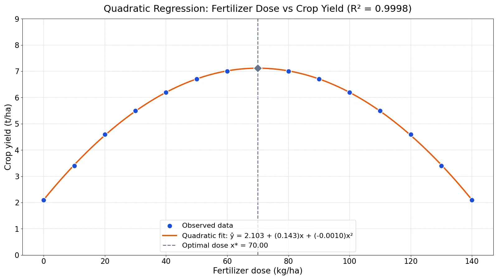
The dataset is 15 fertilizer doses in kg/ha with the resulting crop yield in t/ha, and the response curves upward then downward.

dose (kg/ha)	yield (t/ha)	dose (kg/ha)	yield (t/ha)
0	2.1	80	7.0
10	3.4	90	6.7
20	4.6	100	6.2
30	5.5	110	5.5
40	6.2	120	4.6
50	6.7	130	3.4
60	7.0	140	2.1
70	7.1

The sample size is $n = 15$, the mean dose is $\bar{x} = 70.0000$, and the mean yield is $\bar{y} = 5.2067$.

The design matrix $X = [1, x, x^2]$ has shape (15, 3). The normal equations $X^{\top}X\beta = X^{\top}y$ give a 3 by 3 system on the left and a length-3 vector on the right. Solving yields:

$$a = 2.1032, \quad b = 0.14324, \quad c = -0.0010231$$

So the fitted equation is:

$$\hat{y} = 2.1032 + 0.14324x - 0.0010231x^2$$

At the mean dose $x = 70$:

$$\hat{y} = 2.1032 + (0.14324)(70) + (-0.0010231)(70^2) \approx 7.1165$$

The residual sum of squares is $SS_{res} = 0.0073$ and the total sum of squares is $SS_{tot} = 43.1893$. The coefficient of determination is:

$$R^2 = 1 - \frac{0.0073}{43.1893} = 0.9998$$

The vertex is at:

$$x^* = -\frac{0.14324}{2(-0.0010231)} \approx 70.0000$$

and the predicted yield there is $\hat{y}(x^*) = 7.1165$. Because $c$ is negative, this is a maximum. The model says the best dose in the observed range is about 70 kg/ha, giving roughly 7.12 t/ha.

Here is the code that produces these numbers.

import numpy as np
dose = np.array([0,10,20,30,40,50,60,70,80,90,100,110,120,130,140])
yield_ = np.array([2.1,3.4,4.6,5.5,6.2,6.7,7.0,7.1,7.0,6.7,6.2,5.5,4.6,3.4,2.1])
c, b, a = np.polyfit(dose, yield_, 2)
yhat = np.polyval([c,b,a], dose)
r2 = 1 - ((yield_-yhat)**2).sum()/((yield_-yield_.mean())**2).sum()
print(f"a={a:.4f}, b={b:.4f}, c={c:.4f}, R²={r2:.4f}")

Output:

a=2.1032, b=0.1432, c=-0.0010, R²=0.9998

Other Ways to Do It

In R you can add the squared term directly in the formula. The call lm(y ~ x + I(x^2)) fits the same family of curves as lm(y ~ poly(x, 2)), but the coefficients differ because a different model matrix is used [1]. The fitted values and $R^2$ are identical either way.

In a spreadsheet, add a column of squared $x$ values and run the ordinary least-squares routine on the three columns. That is the same computation as the matrix approach above [3].

If you want to try a quick fit without writing code, the Linear Regression Calculator handles the arithmetic for a straight line, which is a useful first check before you add the squared term.

For a broader view of how this model sits among others, see What is Regression Analysis? A Practical Introduction and the discussion of OLS Regression.

Troubleshooting

The curve fits but the vertex is outside your data range. The formula for $x^*$ always returns a number, but if it falls far outside the observed $x$ values, you are extrapolating. Report it as a mathematical artifact, not a finding.

Coefficients change wildly when you add or remove a point. This is common when the $x$ values are clustered. Spread the doses more evenly and refit.

$R^2$ is high but residuals show a pattern. A high $R^2$ does not prove the model is right. Look at the residual plot before trusting the fit [4].

The linear and quadratic terms look unstable. Centering $x$ by subtracting its mean often reduces the correlation between the $x$ and $x^2$ columns and makes the coefficients easier to read.

Common Mistakes

Reading $b$ as "the effect of $x$." In a quadratic model the slope changes at every point. The marginal effect at a given $x$ is $b + 2cx$. Fix: report the slope at specific values, or report the vertex.
Ignoring the sign of $c$. A positive $c$ means the curve opens upward, so the vertex is a minimum, not a maximum. Fix: always state the direction before interpreting the turning point.
Extrapolating past the data. A parabola keeps rising or falling forever. Fix: restrict predictions to the observed range of $x$.
Trusting coefficient p-values without correction. Each coefficient is tested separately and the tests are not corrected for multiple testing [1]. Fix: treat them as screening tools, not proof.
Assuming a quadratic is always better than a line. Adding a squared term always raises $R^2$ slightly, even for straight data. Fix: compare models on residual plots and adjusted measures, not raw $R^2$ alone.
Forgetting that $x$ and $x^2$ are correlated. This inflates standard errors. Fix: center $x$ before squaring when interpretation matters.

Limitations

A quadratic model has one turning point. Real relationships often have none, or several. If the underlying process is asymptotic, a curve that flattens toward a ceiling, a quadratic will eventually turn back and give nonsense predictions outside the data. For that shape, a nonlinear model is more appropriate [2].

The method also assumes the errors behave reasonably, with roughly constant variance and no strong dependence between observations. When those assumptions fail, the coefficient estimates may still be usable but the intervals and tests can mislead. And a good fit to 15 points does not mean the curve generalizes. The fertilizer example has a near-perfect $R^2$ because the data were generated on a smooth parabola, which is rare in practice. For related modeling choices, see Assumptions of Linear Regression and Generalized Linear Models.

Frequently Asked Questions

What is the quadratic regression equation?

It is $\hat{y} = a + bx + cx^2$. The intercept $a$ is the predicted value when $x = 0$, $b$ controls the initial slope, and $c$ controls the curvature. If $c$ is negative the curve bends downward, and if it is positive the curve bends upward.

How do I find the maximum or minimum?

Use $x^ = -b/(2c)$, then substitute that value into the equation to get the predicted response. In the fertilizer example, $x^ = 70.0000$ kg/ha and the predicted yield is 7.1165 t/ha. Because $c$ is negative, this is a maximum.

Is quadratic regression the same as nonlinear regression?

No. Quadratic regression is linear in the parameters, so it is fitted by ordinary least squares with a design matrix that includes $x^2$ [1]. Nonlinear least squares covers models where parameters enter the function in ways that cannot be written as a linear combination [2].

Can I use more than one predictor?

Yes. You can add squared terms for several predictors and their products, which gives a full second-order surface [1]. The interpretation gets harder because each coefficient depends on the others, so centering the predictors helps.

How many data points do I need?

There is no fixed minimum, but you need enough distinct $x$ values to separate the linear and quadratic parts. Five or six well-spread levels is a practical floor. With fewer, the two terms compete and the coefficients become unstable.