What Is Log-Likelihood? Definition, Formula and Examples

By Dr. Zubair Khalid, DVM, MS, PhD · 2026-10-03

The log-likelihood statistic measures how well a probability model explains the data you actually observed. It is the natural logarithm of the likelihood, the joint probability of the data given a set of parameter values. Higher values (closer to zero, since log-likelihoods are usually negative) mean the model assigns more probability to what you saw.

Quick Answer

The likelihood is the probability of the observed data as a function of the model parameters [1].
The log-likelihood is the natural log of that likelihood, which turns a product of many probabilities into a sum of logs [2].
For independent observations, $l(\theta) = \sum_{i=1}^{n} \log f_\theta(x_i)$, where $f_\theta$ is the probability density or mass for one observation [2].
Maximum likelihood estimation finds the parameter values that make the log-likelihood as large as possible [3].
Log-likelihood values are often negative, and for models fitted to the same data a higher value (closer to zero when negative) indicates a better fit [1].

What the Log-Likelihood Statistic Means

In plain terms, the likelihood asks a simple question: given these parameter values, how probable is the data I collected? A model that makes your data look likely is doing a good job. A model that makes your data look nearly impossible is doing a poor job.

The precise definition starts with the likelihood function. For a data set $x = (x_1, \dots, x_n)$ and a model with parameters $\theta$, the likelihood is the joint probability (or density) of the data treated as a function of $\theta$. When observations are independent and identically distributed, that joint probability is a product of individual terms [2]:

$$L(\theta; x) = \prod_{i=1}^{n} f_\theta(x_i)$$

The log-likelihood is the natural logarithm of $L$:

$$l(\theta; x) = \log L(\theta; x) = \sum_{i=1}^{n} \log f_\theta(x_i)$$

The last step uses the rule that the log of a product equals the sum of the logs [2]. That single fact is why the log-likelihood statistic is used everywhere in model fitting. Multiplying hundreds of small probabilities underflows to zero on a computer, while summing their logs stays numerically stable. Many procedures use the log of the likelihood for exactly this reason [1].

How It Works

Each symbol in the formula carries a specific meaning.

Symbol	Meaning
$x_i$	The $i$-th observed data point
$n$	The number of observations
$\theta$	The parameter or vector of parameters of the model
$f_\theta(x_i)$	The probability density or mass of $x_i$ under parameters $\theta$
$L(\theta; x)$	The likelihood, the joint probability of all data
$l(\theta; x)$	The log-likelihood, the natural log of $L$

To compute it, you evaluate the density of every observation at the candidate parameter values, take the log of each, and add them up [2]. To fit a model, you search over $\theta$ for the value that maximizes this sum. That value is the maximum likelihood estimate [3]. In practice, software minimizes the negative log-likelihood, because minimizing minus the log-likelihood is the same as maximizing the log-likelihood [2].

The log-likelihood also supports extensions. A penalized log-likelihood subtracts a penalty term from the log-likelihood, which pulls estimates toward values grounded in outside information [3]. For complex models where the log-likelihood cannot be computed directly, researchers can estimate it by simulation [4].

Worked Example

Suppose you recorded 20 reaction times (in milliseconds) from a simple lab task and want to fit a normal model.

412	388	455	402	371
430	398	447	415	392
468	405	421	379	441
396	428	410	453	384

You compare two candidate models that share the same standard deviation but differ in their mean. Model A uses the maximum likelihood mean. Model B fixes the mean at 400 ms.

Step 1. Sample size. $n = 20$.

Step 2. MLE mean. $\hat{\mu} = \sum x / n = 8295 / 20 = 414.7500$.

Step 3. MLE standard deviation. Using the divide-by-$n$ form, $\hat{\sigma} = \sqrt{\sum (x - \hat{\mu})^2 / n} = 26.8195$.

Step 4. Log-likelihood for Model A. Summing the normal log-density at $\mu = 414.7500$ and $\sigma = 26.8195$ gives $-94.1614$.

Step 5. Log-likelihood for Model B. Summing the same log-density at $\mu = 400$ gives $-97.1861$.

Step 6. Difference. $-94.1614 - (-97.1861) = 3.0247$. Model A has the higher log-likelihood, so it fits better.

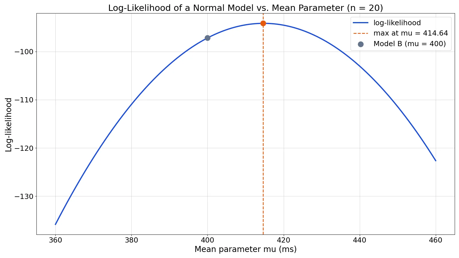
Step 7. Check the peak. Scanning the log-likelihood curve over a grid of $\mu$ values places the highest grid point at $\mu = 414.6366$, next to the exact maximum at the MLE mean of 414.75.

Here is the computation in Python:

from scipy.stats import norm
import numpy as np
rt = [412, 388, 455, 402, 371, 430, 398, 447, 415, 392,
      468, 405, 421, 379, 441, 396, 428, 410, 453, 384]
mu = np.mean(rt)
sd = np.std(rt)  # MLE: divide by n
ll = np.sum(norm.logpdf(rt, loc=mu, scale=sd))
print(round(ll, 4))  # -94.1614

Output:

-94.1614

The figure below shows the log-likelihood of the normal model as a function of the mean parameter, with the maximum marked at $\mu = 414.64$.

How to Interpret It

The absolute value of a log-likelihood is hard to read on its own. It depends on the sample size, the model, and the units of the data. What matters is comparison.

When two models are fitted to the same data, the one with the higher log-likelihood fits better. The difference between two log-likelihoods drives the likelihood ratio test, whose statistic is $LR = 2(\text{loglik}(m_2) - \text{loglik}(m_1))$, where $m_1$ is the more restrictive model and $m_2$ is the less restrictive one [1]. That statistic follows a chi-squared distribution with degrees of freedom equal to the number of constrained parameters [1].

For the same data, a higher log-likelihood means a better fit. Here both values are negative, so the better one is closer to zero. A value of $-94.16$ is better than $-97.19$ for the same data and the same number of parameters.

When to Use It (and when not to)

Use the log-likelihood statistic whenever you fit a model by maximum likelihood, compare nested models, or compute information criteria such as AIC and BIC. It is the foundation of parameter estimation and model evaluation across statistics, epidemiology, and computational fields [3][4]. It also underlies the likelihood ratio, Wald, and score tests, which all use the likelihood of the models being compared [1].

Do not use raw log-likelihood to compare models fitted to different data sets, different sample sizes, or different response variables. The scale changes, so the numbers are not comparable. Do not treat a higher log-likelihood as proof that a model is correct. Maximum likelihood is based on an assumed model and cannot account for bias sources the model or study design does not control [3]. Adding parameters almost always raises the log-likelihood, so a more complex model will look better even when it is not. Use a penalized criterion or a formal test instead.

Log-Likelihood vs Likelihood

The likelihood and the log-likelihood contain the same information, since the log is a monotonic transformation. The parameter value that maximizes one maximizes the other. The difference is practical.

Feature	Likelihood	Log-Likelihood
Form	Product of densities	Sum of log densities
Typical scale	Very small positive numbers	Negative numbers near zero
Numerical stability	Underflows with many observations	Stable
Maximized at	Same $\theta$	Same $\theta$
Used for	Definition and theory	Fitting and comparison

Because the log turns products into sums, it is easier to work with and easier to differentiate when solving for the maximum [1][2].

Common Mistakes

Reading the absolute value as a fit score. A log-likelihood of $-94$ is not "94 percent good." Fix: compare it only against another log-likelihood computed on the same data.
Comparing log-likelihoods across different data sets. The scale depends on the sample and the response variable. Fix: restrict comparisons to models fitted to identical data.
Forgetting that adding parameters inflates the value. More parameters almost always raise the log-likelihood. Fix: use AIC, BIC, or a likelihood ratio test with the correct degrees of freedom [1].
Using the divide-by-$n$ standard deviation when software expects divide-by-$(n-1)$. The two differ, and the log-likelihood changes with the value you plug in. Fix: match the estimator to your model's parameterization.
Assuming a higher log-likelihood proves the model is right. It only says the model assigns more probability to the data. Fix: check assumptions and study design separately [3].
Ignoring numerical problems in complex models. Some log-likelihoods are intractable to compute directly. Fix: use simulation-based estimation when needed [4].

Limitations

The log-likelihood statistic is a relative measure, not an absolute one. It cannot tell you whether your model is correctly specified, only how well it ranks against alternatives on the same data. A model can have the highest log-likelihood among a set of candidates and still be badly wrong if every candidate shares the same flawed assumptions [3].

For some distributions, maximum likelihood methods run into theoretical or numerical problems, such as a solution that does not exist or an algorithm that fails to converge [5]. In complex models, the log-likelihood may be impossible to compute analytically, so you must estimate it, and naive simulation methods can introduce bias [4]. Treat the number as one piece of evidence, not a verdict.

Frequently Asked Questions

Why is the log-likelihood always negative?

It is not always negative. For discrete data, each probability is at most 1, so its log is at most 0 and the log-likelihood can never be positive. For continuous data, densities can exceed 1 when the data are tightly concentrated (for example a normal model with a small standard deviation), so the log-likelihood can be positive. In every case, a higher value indicates a better fit for the same data [1].

What is a good log-likelihood value?

There is no universal threshold. The value depends on sample size, model, and data scale. A "good" value is one that is higher than the log-likelihood of a competing model fitted to the same data. Use differences between log-likelihoods, not the raw number, to judge fit [1].

How is the log-likelihood used to compare models?

Subtract one log-likelihood from another and multiply by 2 to get the likelihood ratio test statistic. Under the null hypothesis that the simpler model is adequate, this statistic follows a chi-squared distribution with degrees of freedom equal to the number of constrained parameters [1]. A large value favors the more complex model.

Does a higher log-likelihood always mean a better model?

No. Adding parameters nearly always increases the log-likelihood, even when the extra terms add no real value. Penalized criteria such as AIC and BIC subtract a complexity penalty to offset this. A penalized log-likelihood does the same thing by shrinking estimates toward outside values [3].

Can I compute the log-likelihood by hand?

For small data sets and simple models, yes. Write down the density for each observation, take the natural log, and add the results. For anything larger, use software. In Python, scipy.stats.norm.logpdf returns the log density, and summing it gives the log-likelihood directly, as in the worked example above.