Cramer's V: Definition, Formula and Examples
By Dr. Zubair Khalid, DVM, MS, PhD ·
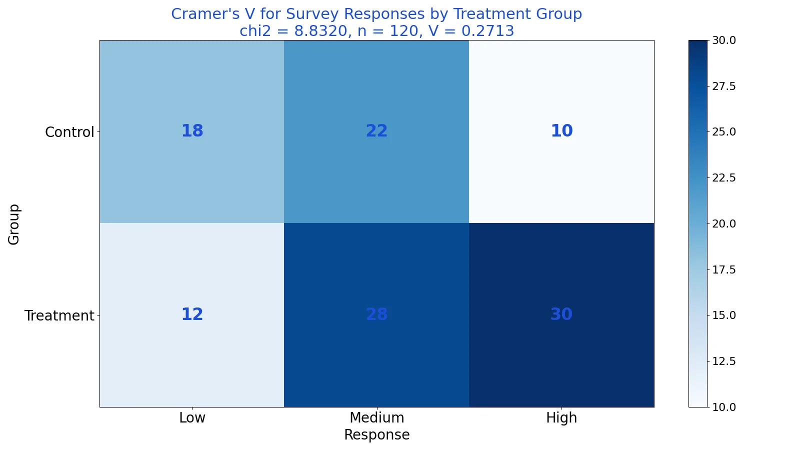
Cramer's V is a measure of association between two categorical variables. It takes a chi-square statistic and converts it into a number between 0 and 1, where 0 means no association and 1 means a perfect association. It works for tables of any size, which makes it the default strength measure after a significant chi-square test [1][2].
Quick Answer
- Cramer's V measures how strongly two categorical variables are related, on a scale from 0 to 1.
- The formula is $V = \sqrt{\dfrac{\chi^2}{n \cdot \min(r-1,\ c-1)}}$, where $\chi^2$ is the chi-square statistic, $n$ is the sample size, and $r$ and $c$ are the table's row and column counts.
- It is symmetric, so it does not assume one variable causes the other [1].
- It applies to nominal, ordinal, or binary variables, though Phi is preferred for two binary variables [1].
- A common rough guide treats values below 0.10 as weak, 0.10 to 0.25 as moderate, and above 0.25 as strong in social science research [3].
What Cramer's V Means
In plain terms, Cramer's V tells you how much knowing one variable's category helps you predict the other variable's category. If every group has the same mix of outcomes, V is near 0. If each category of one variable lines up almost perfectly with one category of the other, V is near 1.
The precise definition: Cramer's V is the square root of the chi-square statistic divided by the product of the sample size and the smaller of (rows minus one) or (columns minus one) [1]. It is a symmetric, non-directional measure, meaning it treats both variables the same way and does not point to a cause [1]. The size of the table and the number of categories in each variable do not change the scale, so you can compare V values across tables with different dimensions [1].
How It Works
The formula is:
$$V = \sqrt{\frac{\chi^2}{n \cdot \min(r-1,\ c-1)}}$$
Each symbol means:
- $\chi^2$ is the chi-square statistic from the test of independence, computed as $\sum \frac{(O-E)^2}{E}$, where $O$ is an observed cell count and $E$ is the expected count under independence.
- $n$ is the total number of observations in the table.
- $r$ is the number of rows.
- $c$ is the number of columns.
- $\min(r-1,\ c-1)$ is the smaller of the two values, which corrects for the table's shape.
The chi-square statistic alone tells you whether an association exists, but its size grows with the sample size, so it cannot measure strength on its own [2]. Dividing by $n$ removes that dependence, and dividing by $\min(r-1,\ c-1)$ rescales the result so the maximum possible value is 1. The square root brings the value back to a linear scale.
Worked Example
A survey records responses (Low, Medium, High) for a Control group and a Treatment group. The contingency table is:
| Group | Low | Medium | High | Row total |
|---|---|---|---|---|
| Control | 18 | 22 | 10 | 50 |
| Treatment | 12 | 28 | 30 | 70 |
| Column total | 30 | 50 | 40 | 120 |
The grand total is $n = 120$. Expected counts come from $E = \frac{\text{row total} \times \text{column total}}{n}$. For the Control/Low cell, $E = \frac{50 \times 30}{120} = 12.5000$, and the cell contribution is $\frac{(18-12.5000)^2}{12.5000} = 2.4200$.
Repeating this for every cell gives:
| Cell | Observed | Expected | $(O-E)^2/E$ |
|---|---|---|---|
| Control, Low | 18 | 12.5000 | 2.4200 |
| Control, Medium | 22 | 20.8333 | 0.0653 |
| Control, High | 10 | 16.6667 | 2.6667 |
| Treatment, Low | 12 | 17.5000 | 1.7286 |
| Treatment, Medium | 28 | 29.1667 | 0.0467 |
| Treatment, High | 30 | 23.3333 | 1.9048 |
Summing the last column gives $\chi^2 = 8.8320$. The degrees of freedom are $(r-1)(c-1) = (2-1)(3-1) = 2$, and the p-value is 0.0121. The smaller of $r-1$ and $c-1$ is 1, so:
$$V = \sqrt{\frac{8.8320}{120 \times 1}} = 0.2713$$
The chi-square test is significant at the 0.05 level, and V of 0.2713 sits just above the 0.25 cutoff, so the rough social science guide used in this article would label it a strong association.
Here is the same calculation in Python:
import numpy as np
from scipy.stats import chi2_contingency
table = np.array([[18,22,10],[12,28,30]])
chi2, p, dof, exp = chi2_contingency(table, correction=False)
n = table.sum()
V = np.sqrt(chi2 / (n * min(table.shape[0]-1, table.shape[1]-1)))
print(f"chi2={chi2:.4f}, p={p:.4f}, dof={dof}, V={V:.4f}")
Output:
chi2=8.8320, p=0.0121, dof=2, V=0.2713How to Interpret It
Cramer's V ranges from 0 to 1. A value of 0 means the two variables are independent, and a value of 1 means one variable is perfectly predicted by the other. There is no universal cutoff, because the meaning of "strong" depends on your field and your variables [4]. One widely used classification in social science research labels V below 0.10 as weak, 0.10 to 0.25 as moderate, and above 0.25 as strong [3].
Two cautions apply when you read a V value. First, always report it alongside the chi-square p-value, since V describes strength while the p-value describes whether the association is likely to be real [2]. Second, remember that a moderate V can still be meaningful in a large sample, and a large V in a tiny sample can be unstable. If you want a sense of the underlying variability, reviewing how a mean and standard deviation behave in your sample can help you judge how much noise to expect.
When to Use It (and when not to)
Use Cramer's V when both variables are categorical and you have already run a chi-square test of independence. It handles nominal, ordinal, and binary variables, and it works for tables larger than 2x2, where Phi is no longer appropriate [1][5]. It is the most common strength measure reported after a significant chi-square result [2].
Avoid it in a few situations. For two binary variables, Phi is the standard choice, even though V returns the same value [1]. For two ordinal variables, measures designed for ordered categories are usually more informative [1]. If your table has a large imbalance between the number of rows and columns, V can overestimate the association [1]. And if your variables are continuous, use a correlation coefficient instead.
Cramer's V vs Phi
Phi and Cramer's V are closely related. Phi is the square root of chi-square divided by the sample size, and it is designed for 2x2 tables [1]. Cramer's V generalizes that idea to larger tables by adding the $\min(r-1,\ c-1)$ correction. For a 2x2 table, the correction equals 1, so the two formulas produce identical values [1][5].
| Feature | Cramer's V | Phi |
|---|---|---|
| Table size | Any r x c table | 2x2 tables |
| Formula | $\sqrt{\chi^2 / (n \cdot \min(r-1, c-1))}$ | $\sqrt{\chi^2 / n}$ |
| Value on a 2x2 table | Same as Phi | Same as V |
| Typical use | Nominal or ordinal pairs, larger tables | Two binary variables |
Common Mistakes
- Reporting V without the chi-square p-value. V measures strength, not significance. Report both so readers know whether the association is likely real [2].
- Using V for a 2x2 table when Phi is expected. The values match, but Phi is the conventional choice for two binary variables [1].
- Treating V as a measure of direction or causation. V is symmetric and non-directional, so it never tells you which variable drives the other [1].
- Comparing V across studies with very different sample sizes without caution. Small samples produce unstable estimates, and a large row-to-column imbalance can inflate V [1].
- Assuming a fixed cutoff for weak, moderate, and strong. Naming conventions vary by field, so state the benchmark you are using [4].
- Forgetting that V ignores category order. If your categories are ordered, V treats them as unordered labels, which can hide a monotonic trend.
Limitations
Cramer's V cannot tell you the direction of an association or which categories drive it. It also cannot establish causation, since a third variable may explain the relationship. Because it depends on the chi-square statistic, it inherits the chi-square assumption that expected counts are large enough for the test to be valid, and sparse tables with many small expected counts can distort the result.
The value of V is also sensitive to table shape. When the number of rows and columns differ substantially, V tends to overestimate the association [1]. For ordinal variables, V ignores the ordering and can understate a real monotonic relationship. Treat V as one piece of evidence alongside the full contingency table, the p-value, and your knowledge of the data.
Frequently Asked Questions
What is a good Cramer's V value?
There is no single threshold. A common social science guide calls values below 0.10 weak, 0.10 to 0.25 moderate, and above 0.25 strong [3]. Other fields use different labels, so report the benchmark you rely on and interpret V in context [4].
Can Cramer's V be negative?
No. Because it is a square root of a non-negative quantity, V ranges from 0 to 1. It measures strength only, so it never carries a sign. If you need direction, examine the individual cell counts or use a directional measure.
What is the difference between Cramer's V and chi-square?
Chi-square tests whether an association exists and grows with sample size. Cramer's V rescales that statistic to a 0-to-1 range so you can judge strength independently of sample size [2]. They are usually reported together.
When should I use Cramer's V instead of Phi?
Use Phi for 2x2 tables and Cramer's V for anything larger [1][5]. On a 2x2 table the two give the same number, but Phi is the conventional label for two binary variables.
Does Cramer's V work for ordinal variables?
It can be computed, but it treats the categories as unordered, so it may miss a monotonic trend [1]. For ordinal pairs, a measure that respects category order is usually a better fit.
References
- 2.5: An In-Depth Look At Measures of Association - Statistics LibreTexts/02%3A_Quantitative_Data_Analysis/2.05%3A_An_In-Depth_Look_At_Measures_of_Association)
- McHugh ML. (2013). The chi-square test of independence. Biochemia medica
- Two Basic Summary Statistics
- Akoglu H. (2018). User's guide to correlation coefficients. Turkish journal of emergency medicine
- lectur15