What Is a Trimmed Mean? Definition, Formula and Examples

By Dr. Zubair Khalid, DVM, MS, PhD · 2026-10-03

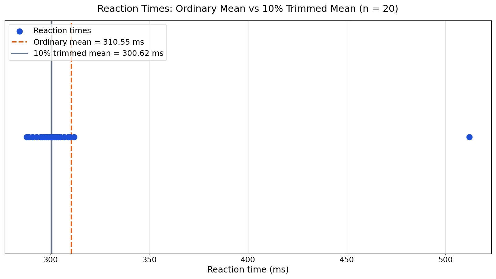
Trimmed means are averages calculated after deleting a fixed percentage of the smallest and largest values from a dataset. They sit between the ordinary mean and the median: more resistant to outliers than the mean, but built from more of the data than the median. This article explains the definition, the formula, a full worked example, and how to compute trimmed means by hand or in code.

Quick Answer

A trimmed mean drops a set percentage of values from each tail of a sorted dataset, then averages the rest.
The trimming proportion is split equally between the low end and the high end, so a 10% trimmed mean removes 10% from the bottom and 10% from the top.
The number trimmed from each end is $k = \lfloor \gamma n \rfloor$, where $\gamma$ is the trim proportion and $n$ is the sample size [1].
Trimming makes the statistic resistant to extreme values, so one wild observation cannot drag the average far off [1].
In the worked example below, the ordinary mean is 310.55 ms and the 10% trimmed mean is 300.625 ms, a gap of 9.925 ms caused by a single slow reaction time.

What a Trimmed Mean Means

A trimmed mean is the ordinary arithmetic mean of a dataset after you have removed a fixed share of the most extreme values from both ends. You sort the data, cut the same number of values off the low tail and the high tail, and average whatever is left.

The precise statistical definition: given a sorted sample $x_{(1)} \le x_{(2)} \le \dots \le x_{(n)}$ and a trimming proportion $\gamma$ with $0 \le \gamma < 0.5$, the trimmed mean is the average of the observations that remain after discarding the lowest $k$ and highest $k$ values, where $k = \lfloor \gamma n \rfloor$ [1]. The trimming fraction is applied to each tail separately, so $\gamma = 0.10$ means 10% off the bottom and 10% off the top [1].

The idea comes from Mosteller and Tukey, who described resistance as the property that changing a small part of the data, even by a large amount, does not cause a large change in the statistic [1]. A trimmed mean has that property. Move the single largest value from 512 to 5,000 and the trimmed mean does not budge, because that value was already excluded.

How It Works

The formula for the trimmed mean is:

$$ \bar{x}_t = \frac{1}{n - 2k} \sum_{i=k+1}^{n-k} x_{(i)} $$

Each symbol means the following.

$x_{(i)}$ is the $i$-th value in the sorted dataset, from smallest to largest.
$n$ is the total number of observations.
$\gamma$ (gamma) is the trimming proportion, the fraction removed from each tail.
$k = \lfloor \gamma n \rfloor$ is the number of values trimmed from each end. The floor function rounds down to a whole number, because you cannot delete part of an observation [1].
$n - 2k$ is the number of values that survive and get averaged.

Two special cases are worth knowing. When $\gamma = 0$, no values are trimmed and the trimmed mean equals the ordinary mean. When $\gamma$ approaches 0.5, the trimmed mean approaches the median, because almost everything except the middle is discarded. Trimming 25% from each tail ($\gamma = 0.25$) gives the mean of the values between the lower and upper quartiles, often called the interquartile mean [1]. Trimming 5% from each tail ($\gamma = 0.05$) averages the middle 90% of the data [1].

If your data arrives as a frequency table, you can apply weights to each value and compute a weighted trimmed mean instead, using the same trimming indices on the sorted response variable [2].

Worked Example

The dataset is 20 reaction times in milliseconds from a simple reaction-time task, including one unusually slow response.

Reaction time (ms)
312
298
305
289
301
295
310
288
302
299
307
293
296
304
300
291
297
303
309
512

Step 1. Count the observations. $n = 20$.

Step 2. Choose the trim proportion. $\gamma = 0.10$, meaning 10% off each tail.

Step 3. Compute how many values to trim from each end.

$$ k = \lfloor 0.10 \times 20 \rfloor = 2 $$

Step 4. Sort the values.

288, 289, 291, 293, 295, 296, 297, 298, 299, 300, 301, 302, 303, 304, 305, 307, 309, 310, 312, 512

Step 5. Remove the lowest 2 values: 288 and 289.

Step 6. Remove the highest 2 values: 312 and 512.

Step 7. Count what remains. $20 - 2 \times 2 = 16$ values.

Step 8. Sum the remaining 16 values: 4810.

Step 9. Divide.

$$ \bar{x}_t = \frac{4810}{16} = 300.6250 $$

For comparison, the ordinary mean uses all 20 values: $6211 / 20 = 310.5500$. The difference is $310.5500 - 300.6250 = 9.9250$ ms. That entire gap comes from the outlier at 512 ms, which sits far above the rest of the data and pulls the ordinary mean upward. The trimmed mean stays close to the bulk of the observations, which cluster around 300 ms.

Here is the same calculation in Python.

import statistics
times = [312, 298, 305, 289, 301, 295, 310, 288, 302, 299,
         307, 293, 296, 304, 300, 291, 297, 303, 309, 512]
n = len(times)
k = int(0.10 * n)
trimmed = sorted(times)[k:n-k]
print(statistics.mean(trimmed))  # 300.6250
print(statistics.mean(times))    # 310.5500

Output:

300.6250
310.5500

You can check the same numbers with a mean, median and mode calculator if you want to compare the trimmed mean against the ordinary mean and the median on your own data.

How to Interpret It

Read a trimmed mean as the typical value of the middle of your data, with the tails deliberately ignored. In the example, 300.625 ms is a better description of how fast this person usually reacts than 310.55 ms, because the ordinary mean is inflated by one slow trial.

The size of the gap between the ordinary mean and the trimmed mean is itself informative. A small gap means the tails are light and the two statistics agree. A large gap means extreme values are doing real work in the ordinary mean, and you should ask whether those values are genuine measurements or errors.

Trimmed means also behave well as estimators. Statisticians describe two desirable properties. Resistance means a small change in a small part of the data does not cause a large change in the statistic. Efficiency means the estimator performs well across a variety of situations instead of in just one [1]. A trimmed mean trades a little efficiency when data are perfectly normal for much better performance when they are not.

When to Use It (and when not to)

Use a trimmed mean when your data contain outliers you cannot justify deleting outright, when the distribution has heavy tails, or when you want a summary that is stable across repeated samples. It is common in economics for inflation measurement, where trimmed mean inflation rates cut off the extreme price changes at both ends of the distribution [3]. It also appears in clinical trials as a way to handle patient dropout, where early discontinuation is treated as a bad outcome and an equal percentage of bad outcomes is trimmed from each treatment arm [4].

Do not use a trimmed mean when every observation matters equally and none should be downweighted. If you are reporting total revenue, the sum and the ordinary mean are the right tools, because a single large customer is a real part of the business. Do not trim when the extremes are the finding. If you are studying the worst-case latency of a system, deleting the slowest responses removes exactly the information you need.

Also avoid trimming when $n$ is very small. With $n = 8$ and $\gamma = 0.10$, $k = \lfloor 0.8 \rfloor = 0$, so nothing is trimmed and you have computed an ordinary mean without realizing it.

Trimmed Mean vs Median

Both statistics resist outliers, and both require sorting. The difference is how much data they keep.

Feature	Trimmed mean	Median
Values used	All except the trimmed tails	One or two middle values
Typical trim	5% to 25% per tail	Effectively 50% per tail
Sensitivity to trimming choice	Changes with $\gamma$	Fixed
Uses information in the tails	Partially, up to the trim point	No
Behaves like	A compromise between mean and median	The center point

The 25% per tail trimmed mean is the mean of the values between the upper and lower quartiles [1], which is close to but not identical to the median. If you want a single middle value with no tuning parameter, use the median. If you want to keep most of your data and still blunt the influence of extremes, use a trimmed mean.

Common Mistakes

Trimming the wrong total percentage. A "10% trimmed mean" removes 10% from each tail, so 20% of the data is gone in total. If you trim 10% overall, you have computed a 5% trimmed mean. Fix: decide whether your percentage is per tail or overall, and state it explicitly.
Rounding $k$ up instead of down. $k$ must be a whole number of observations, and the standard rule rounds down [1]. With $n = 15$ and $\gamma = 0.10$, $k = \lfloor 1.5 \rfloor = 1$, not 2. Fix: apply the floor function before you delete anything.
Forgetting to sort first. Trimming the first and last rows of an unsorted dataset removes arbitrary values, not extremes. Fix: sort ascending, then cut from both ends.
Trimming different amounts from each tail without saying so. Asymmetric trimming is legitimate and sometimes useful, but it changes the meaning of the statistic. Fix: if you trim unequal amounts, report both tail percentages separately [5].
Comparing trimmed means computed with different trim levels. A 5% trimmed mean and a 25% trimmed mean are different statistics and are not directly comparable. Fix: hold $\gamma$ constant across groups you compare.
Assuming the trimmed mean fixes bad data. Trimming hides the influence of an outlier, it does not tell you whether the outlier is an error. Fix: inspect the trimmed values before you discard them.

Limitations

A trimmed mean discards information by design. If the extreme values in your dataset are real and meaningful, trimming produces a number that describes a population you did not sample. It also introduces a choice that the ordinary mean does not have: you must pick $\gamma$, and different choices give different answers. There is no single correct trim level, only conventions within a field.

Inference is more involved than for the ordinary mean. Standard errors for trimmed means require their own formulas, and confidence intervals are typically built with a t-based approach or a bootstrap method [1]. Software support varies, and some tools require you to specify the lower and upper trim percentages as separate parameters [5]. If you need a simple, widely supported summary, the ordinary mean or the median will usually be easier to defend.

Frequently Asked Questions

What is a 10% trimmed mean?

It is the average of a dataset after removing the lowest 10% and the highest 10% of values. With 20 observations, that means deleting the 2 smallest and 2 largest values and averaging the remaining 16. In the reaction-time example, the 10% trimmed mean is 300.625 ms against an ordinary mean of 310.55 ms.

Is a trimmed mean the same as a winsorized mean?

No. A trimmed mean deletes the extreme values and averages what is left. A winsorized mean replaces the extreme values with the nearest retained value instead of deleting them, so the sample size stays the same. The two are related but produce different numbers.

How do I choose the trim percentage?

Common choices are 5%, 10%, 20%, and 25% per tail. Higher trim levels give more resistance to outliers but use less of your data. A practical approach is to compute the trimmed mean at several levels and check whether the answer is stable. If it barely moves between 5% and 20%, the choice does not matter much for your conclusion.

Can a trimmed mean be used with weighted data?

Yes. When your data is in the form of a frequency table, you can apply weights and compute a weighted trimmed mean, using the same trimming indices on the sorted response variable [2]. The weights must be non-negative and at least one must be positive [2].

Why do economists use trimmed means for inflation?

Trimmed mean inflation measures cut off the largest price increases and decreases each period, which filters out volatile one-off shocks. Research from the Dallas Fed found that first-release trimmed mean inflation tracked headline inflation more closely than first-release core inflation over 2005 to 2018, and that it was generally a better predictor of where inflation was heading [3].