KL Divergence: Definition, Formula and Examples

By Dr. Zubair Khalid, DVM, MS, PhD · 2026-10-03

KL divergence is a number that measures how much one probability distribution differs from another. It tells you the average extra cost, in information terms, of using an approximate distribution $Q$ when the true distribution is $P$. It is widely used in machine learning, statistics and information theory, and its most famous property is that it is asymmetric: $D(P \| Q)$ is usually not equal to $D(Q \| P)$.

Quick Answer

KL divergence, written $D(P \| Q)$, measures the information lost when $Q$ is used to approximate $P$.
The formula is $D(P \| Q) = \sum_i P(i) \ln \dfrac{P(i)}{Q(i)}$ for discrete distributions.
It is always greater than or equal to zero, and equals zero only when $P$ and $Q$ are identical.
It is asymmetric, so $D(P \| Q) \neq D(Q \| P)$ in general.
It is not a distance metric because it fails symmetry and the triangle inequality.

What KL Divergence Means

In plain terms, KL divergence answers this question: if the real data follows distribution $P$, how surprised will I be on average if I model it with distribution $Q$? The more the two distributions disagree, the larger the divergence.

The precise statistical definition is the expected value of the log ratio of the two probability mass functions, taken with respect to $P$:

$$D(P \| Q) = \sum_{i} P(i) \ln \frac{P(i)}{Q(i)}$$

The name honors Solomon Kullback and Richard Leibler, who introduced it in 1951. You will see it written as Kullback-Leibler divergence, KL divergence, or Kullback-Leibler distance, though "distance" is misleading because the measure is not symmetric. The notation $D(P \| Q)$ uses a double vertical bar to signal that the two arguments play different roles.

How It Works

The formula has three moving parts. Each one matters.

$P(i)$ is the probability of outcome $i$ under the reference or true distribution.
$Q(i)$ is the probability of the same outcome under the approximating distribution.
$\ln$ is the natural logarithm, which makes the result measured in nats. If you use $\log_2$ instead, the result is measured in bits.

The ratio $\dfrac{P(i)}{Q(i)}$ compares the two probabilities for a single outcome. When $P(i) > Q(i)$, the ratio is above 1 and its log is positive, so that outcome adds a positive amount. When $P(i) < Q(i)$, the log is negative and the term subtracts. Each term is then weighted by $P(i)$, so outcomes that are common under the true distribution count more.

For continuous distributions, the sum becomes an integral:

$$D(P \| Q) = \int p(x) \ln \frac{p(x)}{q(x)}\, dx$$

Two properties follow directly from the formula. First, $D(P \| Q) \geq 0$ always, a result known as Gibbs' inequality. Second, $D(P \| Q) = 0$ if and only if $P(i) = Q(i)$ for every outcome. If $Q(i) = 0$ for some outcome where $P(i) > 0$, the divergence is infinite, because you assigned zero probability to something that actually happens.

Worked Example

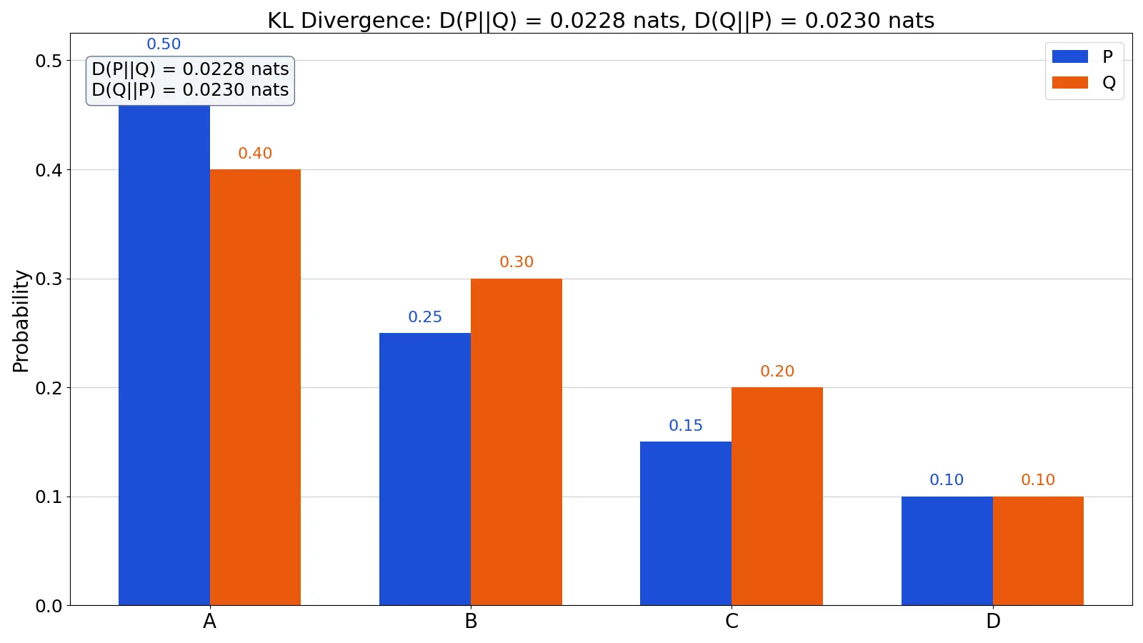
Consider two discrete probability distributions $P$ and $Q$ over four outcomes A, B, C and D. This could represent, for example, the observed click rates on four website buttons ($P$) versus the rates a model predicts ($Q$).

Outcome	P	Q
A	0.5	0.4
B	0.25	0.3
C	0.15	0.2
D	0.1	0.1

To compute $D(P \| Q)$, work through each outcome.

Term 1: $0.5000 \times \ln(0.5000 / 0.4000) = 0.1116$
Term 2: $0.2500 \times \ln(0.2500 / 0.3000) = -0.0456$
Term 3: $0.1500 \times \ln(0.1500 / 0.2000) = -0.0432$
Term 4: $0.1000 \times \ln(0.1000 / 0.1000) = 0.0000$

Summing the terms gives $0.1116 + (-0.0456) + (-0.0432) + 0.0000 = 0.0228$ nats. So $D(P \| Q) = 0.0228$.

Now reverse the arguments to compute $D(Q \| P)$. Each term is now weighted by $Q$ and the ratio is flipped.

Term 1: $0.4000 \times \ln(0.4000 / 0.5000) = -0.0893$
Term 2: $0.3000 \times \ln(0.3000 / 0.2500) = 0.0547$
Term 3: $0.2000 \times \ln(0.2000 / 0.1500) = 0.0575$
Term 4: $0.1000 \times \ln(0.1000 / 0.1000) = 0.0000$

The sum is $-0.0893 + 0.0547 + 0.0575 + 0.0000 = 0.0230$ nats. So $D(Q \| P) = 0.0230$.

The two values differ by $0.0001$ nats. That small gap is the asymmetry in action. The same two distributions give a different divergence depending on which one you treat as the reference.

You can reproduce both numbers with a few lines of Python.

import numpy as np
from scipy.stats import entropy
P = np.array([0.5, 0.25, 0.15, 0.10])
Q = np.array([0.4, 0.30, 0.20, 0.10])
print(entropy(P, Q))  # 0.0228
print(entropy(Q, P))  # 0.0230

Output:

0.02283907559084889
0.02297546100285886

The same calculation works in a spreadsheet. With $P$ in one range and $Q$ in another, the formula =SUMPRODUCT(P_range, LN(P_range/Q_range)) returns 0.0228 for $D(P \| Q)$ and 0.0230 for $D(Q \| P)$.

How to Interpret It

The value is measured in nats when you use the natural log. A divergence of 0.0228 nats is small, which matches what the table shows: $P$ and $Q$ are close but not identical. The largest single contribution came from outcome A, where $P$ is 0.5 and $Q$ is only 0.4. That is the outcome where the model most underestimates the truth, so it carries the most penalty.

There is no universal threshold for "large" or "small." The scale depends on the number of outcomes and the units. What you can do is compare divergences across models on the same data. If model $Q_1$ gives $D(P \| Q_1) = 0.0228$ and model $Q_2$ gives $D(P \| Q_2) = 0.5$, then $Q_1$ is the better approximation of $P$ under this measure.

The direction matters for interpretation. $D(P \| Q)$ penalizes outcomes that are likely under $P$ but unlikely under $Q$. It does not heavily penalize outcomes that $Q$ thinks are likely but $P$ considers rare. If you care about not missing real events, choose the direction that punishes those misses.

When to Use It (and when not to)

Use KL divergence when you have a reference distribution and want to measure how well another distribution approximates it. Common cases include comparing a fitted model to empirical frequencies, measuring the information gain from new data, and as a loss term in training models such as variational autoencoders.

It also appears inside other quantities. Mutual information is a KL divergence between a joint distribution and the product of its marginals. Cross-entropy differs from KL divergence by the entropy of $P$, so minimizing one over $Q$ minimizes the other.

Do not use it when you need a true distance. If you need symmetry and the triangle inequality, use the Jensen-Shannon divergence or the total variation distance. Do not use it when $Q$ can assign zero to an outcome that $P$ allows, because the result becomes infinite. And do not compare raw KL values across datasets with different numbers of categories, since the scale changes.

KL Divergence vs Cross-Entropy

Cross-entropy and KL divergence are closely related, and people often confuse them. The relationship is:

$$H(P, Q) = H(P) + D(P \| Q)$$

where $H(P, Q)$ is the cross-entropy and $H(P)$ is the entropy of $P$.

Property	KL Divergence	Cross-Entropy
Formula	$\sum P \ln(P/Q)$	$-\sum P \ln Q$
Minimum value	0	$H(P)$
Symmetric	No	No
Depends on $P$ alone	No	Yes, through $H(P)$
Typical use	Measuring approximation gap	Training classifiers

When $P$ is fixed, the two differ by a constant, so optimizing one is the same as optimizing the other. KL divergence isolates the part that comes from the mismatch between the distributions.

Common Mistakes

Treating KL divergence as a distance. It is not symmetric and does not satisfy the triangle inequality. Fix: call it a divergence, and always state the direction, as in $D(P \| Q)$.
Swapping the arguments by accident. $D(P \| Q)$ and $D(Q \| P)$ answer different questions. Fix: decide which distribution is the reference before you compute, and label the result.
Using the wrong logarithm base. Natural log gives nats, base 2 gives bits. Fix: state the unit, and stay consistent when comparing values.
Ignoring zero probabilities. If $Q(i) = 0$ where $P(i) > 0$, the divergence is infinite. Fix: smooth $Q$ with a small positive value, or reconsider the model.
Comparing values across different category counts. A distribution over 100 outcomes will generally show larger divergence than one over 4. Fix: compare only on the same outcome space.
Assuming a small value means the model is good. A low divergence in one direction can hide large errors in the other. Fix: check both directions when the application is sensitive to them.

Limitations

KL divergence is unbounded above, so a single value tells you little on its own. It has no fixed maximum, which makes it hard to interpret as a percentage or a score. It also requires both distributions to be defined over the same outcome space, and it breaks down when the approximating distribution assigns zero probability to an event that can occur.

The asymmetry is a feature, not a bug, but it means you must choose a direction deliberately. That choice encodes a value judgment about which errors matter more. The measure also says nothing about where the distributions differ, only how much overall. If you need to know which outcomes drive the gap, inspect the individual terms as in the worked example.

Frequently Asked Questions

Is KL divergence always positive?

Yes. Gibbs' inequality guarantees $D(P \| Q) \geq 0$ for any two distributions. It equals zero only when $P$ and $Q$ are identical everywhere. If you ever compute a negative value, you have made an arithmetic error or swapped a ratio.

Why is KL divergence asymmetric?

The formula weights each term by $P(i)$, the probability under the first argument. When you swap the arguments, you weight by $Q(i)$ instead and flip each ratio. Those are different weighted sums, so the results generally differ. In the worked example, $D(P \| Q) = 0.0228$ and $D(Q \| P) = 0.0230$.

What is the difference between KL divergence and cross-entropy?

Cross-entropy equals the entropy of $P$ plus the KL divergence. When $P$ is fixed, the entropy term is constant, so minimizing cross-entropy is the same as minimizing KL divergence. Cross-entropy is the more common loss function in classification because it avoids computing $H(P)$ separately.

Can KL divergence be infinite?

Yes. If $Q(i) = 0$ for some outcome where $P(i) > 0$, the ratio $P(i)/Q(i)$ is undefined and the divergence goes to infinity. This means the model $Q$ rules out something that actually happens. In practice you avoid this by smoothing or by using distributions with full support.

What units is KL divergence measured in?

It depends on the logarithm base. Natural log gives nats, base 2 gives bits, and base 10 gives hartleys. Most machine learning work uses nats. The worked example above reports 0.0228 nats because it uses the natural logarithm.

References

This article draws on the standard references listed under Further Reading.