Excel Keyboard Shortcuts: Essential Hotkeys for Analysts

By Dr. Zubair Khalid, DVM, MS, PhD · 2026-10-03

Excel keyboard shortcuts are key combinations that let you move around a sheet, select ranges, and edit cells without touching the mouse. The ones that save the most time for analysts are the navigation keys (Ctrl+Arrow), the selection keys (Ctrl+Shift+Arrow), and the editing keys (F2, Alt+=, Ctrl+Shift+L). This guide lists the shortcuts worth memorizing, shows them on a real sheet, and covers the mistakes that trip people up.

Quick Answer

Move to the edge of data: Ctrl+Arrow jumps to the last non-empty cell in that direction.
Select a whole block: Ctrl+Shift+Arrow extends the selection to the edge of the data.
Edit in place: F2 puts the cursor inside the active cell so you can change part of a formula.
Add a total fast: Alt+= inserts AutoSum for the range above or to the left.
Turn filters on and off: Ctrl+Shift+L toggles filter arrows on the header row.

Before You Start

A few ground rules keep these shortcuts predictable.

The shortcuts here refer to the US keyboard layout, and keys on other layouts might not line up exactly with a US keyboard [1]. If your keyboard is set to another language, test each shortcut once before you rely on it.

A plus sign in a shortcut means press the keys at the same time. A comma means press them in order [1]. So Ctrl+Shift+L is three keys held together, while a sequence like Alt, H, O would be pressed one after another.

Excel is available on Windows, Mac, iPad, iPhone, Android tablets and phones, and Excel Mobile [1]. The shortcuts in this article are the Windows set. Mac versions often swap Ctrl for Command, so check the Mac list if you work on a Mac.

If an action you use often has no shortcut, you can record a macro to create one [1]. That is the escape hatch when a repeated task has no built-in key.

Step by Step

These are the shortcuts grouped by what you are trying to do. Practice them in order and they build on each other.

Jump to the edge of your data. Press Ctrl+Arrow. From a cell in a column of values, Ctrl+Down takes you to the last filled cell before a blank. This is the fastest way to reach the bottom of a long list.
Select from here to the edge. Hold Ctrl+Shift and press the same arrow. The selection extends to the last non-empty cell. Repeat the arrow to keep going past blanks.
Select the whole current region. Press Ctrl+A once inside a block of data to select the surrounding region. Press it again to select the entire sheet.
Edit the active cell. Press F2. The cursor moves into the cell so you can change one part of a formula instead of retyping it.
Insert AutoSum. Press Alt+=. Excel proposes a SUM formula for the numbers above or to the left, and you confirm with Enter.
Toggle filters. Press Ctrl+Shift+L with a cell in your header row. Filter arrows appear, and pressing it again removes them.
Open the function list. Start typing a formula and press Tab to accept the suggested function name, or use the formula bar to see the arguments as you type.
Copy a formula down. Select the cell with the formula, copy it, select the destination range, and paste. Relative references adjust for each row.

For a wider walkthrough of turning raw columns into answers, see how to analyse data in Excel step by step.

Worked Example

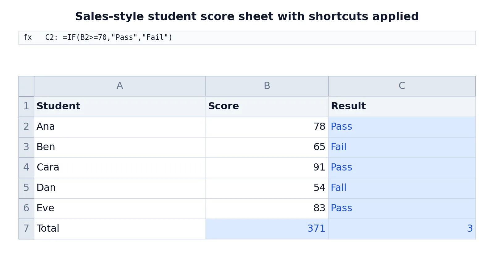
Here is a small score sheet with five students. Column A holds names, column B holds scores, and column C holds a Pass or Fail result from an IF formula.

	A	B	C
1	Student	Score	Result
2	Ana	78	`=IF(B2>=70,"Pass","Fail")` -> displays Pass
3	Ben	65	`=IF(B3>=70,"Pass","Fail")` -> displays Fail
4	Cara	91	`=IF(B4>=70,"Pass","Fail")` -> displays Pass
5	Dan	54	`=IF(B5>=70,"Pass","Fail")` -> displays Fail
6	Eve	83	`=IF(B6>=70,"Pass","Fail")` -> displays Pass
7	Total	`=SUM(B2:B6)` -> displays 371	`=COUNTIF(C2:C6,"Pass")` -> displays 3

The IF formula returns Pass when the score is 70 or above, otherwise Fail. The SUM in B7 totals the five scores to 371, and the COUNTIF in C7 counts how many students passed, which is 3.

Now walk the same sheet with shortcuts only.

Click B2, then press Ctrl+Shift+Down. This selects the range B2:B6, the whole Score column, ready for editing.
With B2:B6 selected, press Alt+= to insert AutoSum in B7. Excel totals the selected scores and shows 371.
Select A1:C6 and press Ctrl+Shift+L. Filter arrows appear on the header row, so you can sort and filter by Result. Selecting only A1:C6 keeps the Total row out of the filter range.
Click the Result filter arrow and choose Pass. Only the passing students stay visible.
Read C7. The COUNTIF still counts 3 passes, because it counts the values in C2:C6.

The figure below shows the same idea: using Ctrl+Arrow, Ctrl+Shift+L, and Alt+= to navigate, filter, and total a small score sheet.

The point of the example is that three shortcuts do most of the work. Ctrl+Shift+Arrow builds the range, Alt+= totals it, and Ctrl+Shift+L turns the header into a filter. The formulas themselves are ordinary. If you want the full syntax behind the result column, see IF AND statements in Excel, and for conditional totals see Excel SUMIF and SUMIFS.

Other Ways to Do It

Shortcuts are one route to the same result. Here are the alternatives and when they are better.

The mouse. Dragging to select a range is fine for a few cells. It gets slow and imprecise once the range runs past one screen.
The Name Box. Type a range like B2:B6 into the Name Box and press Enter to select it exactly. This beats Ctrl+Shift+Arrow when your data has blank rows in the middle.
Go To Special. Use it to select blanks, formulas, or constants in one pass. It is the right tool when you need to select by what a cell contains, not by where it sits.
The filter menu. Clicking the filter arrow works the same as Ctrl+Shift+L once filters are on. The shortcut only saves the trip to the ribbon.
The Quick Access Toolbar. You can customize it with a keyboard, which helps for commands you run constantly but that have no default key [2].

For pulling a subset of rows into a new range, the Excel FILTER function does in one formula what filtering and copying does in several steps.

Troubleshooting

Ctrl+Arrow stops too early. It stops at the last non-empty cell before a blank. If your data has blank rows, it stops early. Use the Name Box or Ctrl+Shift+End to reach the true end of the used range.

Ctrl+Shift+L does nothing. You need a cell inside the header row, or a cell in the data region, for the toggle to apply. If the sheet is protected, filters cannot be added.

Alt+= inserts the wrong total. AutoSum guesses the range above or to the left. If the guess is wrong, drag to correct the range before pressing Enter.

F2 does not enter edit mode. Some keyboards map F2 to another function. Check your keyboard settings if the key does nothing in Excel.

A shortcut works on one machine and not another. Keyboard layout is the usual cause. The shortcuts in the official list refer to the US layout, and other layouts might not correspond exactly [1].

Common Mistakes

Selecting with the mouse when Ctrl+Shift+Arrow would do it. The fix is to click the first cell and extend with the keyboard. It is faster and it lands exactly on the last filled cell.
Typing a formula over a cell you meant to edit. Press F2 first, or click the formula bar. Retyping a long formula to change one number wastes time and invites errors.
Forgetting that filters hide rows, not delete them. The fix is to check the row numbers. Hidden rows still exist, and formulas like SUM over the full range still include them unless you use a filtered-aware function.
Assuming AutoSum picked the right range. The fix is to look at the highlighted range before pressing Enter. If it is wrong, drag to fix it.
Using Ctrl+Arrow inside a filtered list and expecting visible rows only. The fix is to remember that navigation follows the sheet, not the filter. Use visible-cell selection when you need filtered rows only.
Memorizing shortcuts without practicing them in context. The fix is to pick two or three and use them for a week. They stick when they replace a habit you already have.

Limitations

Keyboard shortcuts change what you can do quickly, not what Excel can compute. They will not fix a wrong range, a broken reference, or a formula that points at the wrong column. If the underlying logic is wrong, the shortcut just gets you to the wrong answer faster.

The official shortcut list is written for the US keyboard layout, and keys on other layouts might not correspond exactly [1]. Shortcuts also differ across platforms, so a key that works in Excel for Windows may not work the same way in Excel for Mac or on a tablet [1]. When an action you use often has no shortcut, recording a macro is the documented way to create one [1].

Frequently Asked Questions

What is the most useful Excel keyboard shortcut for analysts?

Ctrl+Shift+Arrow is the one most analysts reach for first. It selects a whole block of data in one motion, which is the starting point for totaling, filtering, or copying. Pair it with Alt+= and you can build a total in two keystrokes.

How do I select a column of data without dragging?

Click the first cell in the column, then press Ctrl+Shift+Down. The selection extends to the last non-empty cell before a blank. If your data has gaps, type the exact range into the Name Box instead.

Why does Ctrl+Arrow stop before the end of my data?

It stops at the last filled cell before a blank row or column. That is by design, since it treats blanks as boundaries. To reach the true end of the used range, use Ctrl+Shift+End.

Can I create my own Excel shortcut?

Yes, if an action you use often has no shortcut key, you can record a macro to create one [1]. That is the documented route for custom keys. For built-in commands, you can also customize the Quick Access Toolbar using the keyboard [2].

Do these shortcuts work the same on Mac?

Not always. The Windows and Mac shortcut sets differ, and the official list is written for the US keyboard layout [1]. On Mac, many combinations use Command where Windows uses Ctrl. Check the Mac section of the official list before relying on a key.

How do I turn filters on and off with the keyboard?

Press Ctrl+Shift+L with a cell in your header row. Filter arrows appear on the header, and pressing the same combination again removes them. Once filters are on, you can open a filter menu and choose values to show.