Excel RIGHT Function: Syntax, Examples and Uses

By Dr. Zubair Khalid, DVM, MS, PhD · 2026-10-03

The Excel RIGHT formula returns the last character or characters in a text string, based on the number of characters you specify [1]. If you have product codes, account numbers or file names and you only need the tail end, RIGHT gives you that slice without any manual editing. This article covers the syntax, a worked example on real product codes, common errors and the limits you should know about.

Quick Answer

RIGHT extracts characters from the end of a text string, counting from the right.
Syntax: =RIGHT(text, [num_chars]).
text is required. num_chars is optional and defaults to 1 if you leave it out [1].
num_chars must be zero or greater. If it is larger than the string length, RIGHT returns the whole string [1].
The result is always text, even when the extracted characters look like numbers.

Syntax

Argument	Required?	Meaning
`text`	Required	The text string containing the characters you want to extract [1].
`num_chars`	Optional	The number of characters you want RIGHT to extract [1].

The function returns a text value. If num_chars is omitted, Excel assumes 1 [1]. If num_chars is greater than the length of text, RIGHT returns all of text [1]. If num_chars is zero, the result is an empty string.

In formal terms, for a string $s$ of length $n$ and a count $k$, RIGHT returns the substring:

$$RIGHT(s, k) = s[n-k+1 \ldots n], \quad 0 \le k \le n$$

When $k > n$, the function returns $s$ in full.

How It Works

RIGHT counts backward from the final character. In the string AB-1042, the last character is 2, the second-to-last is 4, and so on. Asking for 4 characters walks back four positions and returns 1042.

Two behaviors matter in practice. First, RIGHT does not care what the characters are. Letters, digits, spaces, hyphens and punctuation all count as one character each. Second, the output is text. =RIGHT("AB-1042",4) returns the text 1042, not the number 1042. That distinction shows up when you try to sort, sum or compare the result.

If you need to find where a suffix starts before extracting it, pair RIGHT with a position function. The Excel FIND function locates a character's position, and you can feed that position into a length calculation. For converting the extracted text into a formatted value, the Excel TEXT function handles number and date formatting.

Worked Example

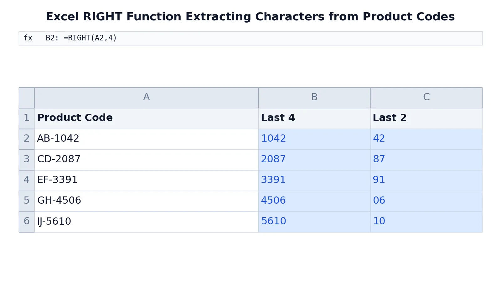
The table below uses a small product code list. Column A holds the codes, column B extracts the last 4 characters and column C extracts the last 2.

	A	B	C
1	Product Code	Last 4	Last 2
2	AB-1042	`=RIGHT(A2,4)` -> displays 1042	`=RIGHT(A2,2)` -> displays 42
3	CD-2087	`=RIGHT(A3,4)` -> displays 2087	`=RIGHT(A3,2)` -> displays 87
4	EF-3391	`=RIGHT(A4,4)` -> displays 3391	`=RIGHT(A4,2)` -> displays 91
5	GH-4506	`=RIGHT(A5,4)` -> displays 4506	`=RIGHT(A5,2)` -> displays 06
6	IJ-5610	`=RIGHT(A6,4)` -> displays 5610	`=RIGHT(A6,2)` -> displays 10

Using =RIGHT(A2,4) and =RIGHT(A2,2) to pull the last four and last two characters from product codes.

Each formula reads the code in column A and returns the trailing characters. In row 5, =RIGHT(A5,2) returns 06, and the leading zero is preserved because the result is text. That is a useful property for codes where leading zeros carry meaning.

More Examples

Extract a file extension. If cell A1 holds report_final.xlsx, the formula =RIGHT(A1,4) returns xlsx. This works when every extension has the same length. For variable-length extensions, you need to locate the dot first.

Extract the last word after a delimiter. Suppose A1 holds North-Region-West. The formula =RIGHT(A1,LEN(A1)-FIND("@",SUBSTITUTE(A1,"-","@",LEN(A1)-LEN(SUBSTITUTE(A1,"-",""))))) returns West. The nested SUBSTITUTE and FIND work finds the position of the final hyphen, and RIGHT takes everything after it.

Combine RIGHT with LEN for dynamic counts. If you want everything except the first 3 characters, use =RIGHT(A1,LEN(A1)-3). This adapts to any string length instead of hard-coding a count.

Convert the result to a number. Wrap the function in VALUE: =VALUE(RIGHT(A2,4)). This turns the text 1042 into the number 1042 so you can sum or average it. The Excel SUM function then works normally on the converted column.

Use RIGHT inside a conditional. =IF(RIGHT(A2,2)="42","Match","No match") tests the suffix. The IF AND statements in Excel guide covers combining multiple conditions, and the IFS function handles longer branching logic.

Look up a value by suffix. If you need to match an extracted suffix against a list, the Excel MATCH function returns the relative position of that value. This is common when codes share a prefix but differ in the tail.

Errors and How to Fix Them

#VALUE! error. This appears when num_chars is negative. RIGHT requires a count of zero or greater [1]. Check the argument and remove the minus sign.

#NAME? error. Usually a misspelled function name or a missing quotation mark around a literal string. Verify the spelling is RIGHT and that text literals are wrapped in double quotes.

Unexpected empty result. If num_chars is 0, RIGHT returns an empty string. Confirm the count is at least 1.

Numbers losing leading zeros. If you extract 06 and Excel treats it as a number, the zero disappears. Keep the result as text or apply a custom number format if you need it displayed with the zero.

Wrong characters returned. This happens when the source string has trailing spaces. Use TRIM first: =RIGHT(TRIM(A2),4). Trailing spaces count as characters and shift the extraction window.

Common Mistakes

Forgetting that the result is text. RIGHT always returns text, so =RIGHT(A2,4)+0 is needed before arithmetic. Fix: wrap in VALUE or add zero.
Hard-coding a count that varies. Using =RIGHT(A1,4) on strings with different suffix lengths returns wrong slices. Fix: compute the count with LEN and a position function.
Ignoring trailing spaces. A cell that looks like AB-1042 may actually be AB-1042 . Fix: apply TRIM before extracting.
Confusing RIGHT with RIGHTB. RIGHTB is deprecated, and RIGHT now supports Unicode surrogates through the Compatibility Version, Version 2 [1]. Fix: use RIGHT for modern work.
Assuming RIGHT works on numbers directly. Numbers are converted to text first, which can change formatting. Fix: format the source as text when leading zeros matter.
Using RIGHT when LEFT or MID fits better. RIGHT only reads from the end. Fix: use LEFT for prefixes and MID for middle segments.

Limitations

RIGHT cannot search for a delimiter on its own. It only counts characters from the end, so if the suffix length varies, you must supply the count from another calculation. It also cannot return multiple separate segments in one call, and it does not handle arrays of strings natively in older Excel versions without entering the formula as an array.

The function returns text, which misleads people who expect numbers. A column of extracted IDs may look numeric but sort as text, and leading zeros may be lost if the value is later coerced to a number. For structured extraction across many rows, a dedicated text-parsing step or a different tool may be more reliable. If you work with tabular data regularly, the tabular data analysis guide covers how to plan these transformations before they cause downstream errors.

Frequently Asked Questions

What does the Excel RIGHT formula do?

It returns the last character or characters in a text string, based on the number of characters you specify [1]. You give it a string and a count, and it reads backward from the end. It is the mirror image of LEFT, which reads from the start.

Is num_chars required in RIGHT?

No. num_chars is optional, and if you omit it, Excel assumes 1 [1]. So =RIGHT(A2) returns just the final character of the string in A2. You only need to supply a count when you want more than one character.

What happens if num_chars is larger than the string?

RIGHT returns all of the text [1]. For example, =RIGHT("AB",5) returns AB because there are only two characters available. No error is raised, which can hide mistakes if your count is wrong.

Why does RIGHT return text instead of a number?

The function is designed for text extraction, so the output is always a text value. If you need to calculate with the result, convert it with VALUE or by adding zero. This behavior is what preserves leading zeros in codes like 06.

Can RIGHT extract text after a specific character?

Not by itself. RIGHT only counts from the end, so you must find the character's position first with FIND or SEARCH, then calculate the remaining length. A common pattern combines LEN, FIND and RIGHT to isolate everything after the last delimiter.

References

RIGHT function | Microsoft Support

References

Further Reading
- Broman KW, Woo KH (2018). Data Organization in Spreadsheets. The American Statistician
- Ziemann M, Eren Y, El-Osta A (2016). Gene name errors are widespread in the scientific literature. Genome Biology
- Microsoft Support: Excel help and learning
- McCullough B, Heiser DA (2008). On the accuracy of statistical procedures in Microsoft Excel 2007. Computational Statistics & Data Analysis
- Abeysooriya M, Soria M, Kasu MS et al. (2021). Gene name errors: Lessons not learned. PLOS Computational Biology
Related Articles
- SQL RIGHT Function: Syntax, Examples and Use Cases
- Excel FIND Function: Syntax, Examples and SEARCH Comparison
- Excel INDIRECT Function: Syntax and Examples
- Excel TEXT Function: Syntax, Format Codes and Examples
- IF AND Statements in Excel: Syntax and Examples
- Pivot Table in Excel: Step-by-Step Tutorial
- Tabular Data: What It Is and How to Analyze It
- Statistical Symbols and Notation: A Quick Reference