Excel FILTER Function: Syntax and Examples

By Dr. Zubair Khalid, DVM, MS, PhD · 2026-10-03

The Excel FILTER function returns only the rows of a range that meet a condition you set. You give it an array to filter and a logical test, and it spills the matching rows into the cells below and to the right of the formula. It is one of the dynamic array functions, so a single formula can return a whole block of results.

Quick Answer

FILTER takes an array and an include argument, and returns the rows where the include test is TRUE.
Syntax: =FILTER(array, include, [if_empty]).
The include argument must be a logical array with the same height or width as the array you are filtering.
Results spill automatically. The formula lives in one cell and fills the neighboring cells.
If no rows match, FILTER returns a #CALC! error unless you supply the optional if_empty value.

Syntax

Argument	Required?	Meaning
`array`	Yes	The range or array you want to filter.
`include`	Yes	A logical array (TRUE/FALSE) that marks which rows or columns to keep. Its height or width must match the array.
`if_empty`	No	The value to return when no rows match the condition.

The function returns an array. In a version of Excel that supports dynamic arrays, that array spills into the surrounding cells. The include argument is usually a comparison such as B2:B6>500, which produces TRUE for rows that pass and FALSE for rows that fail.

How It Works

FILTER walks through the include array row by row. Wherever the test is TRUE, it keeps the corresponding row from array. Wherever the test is FALSE, it drops that row. The kept rows are stacked into a new array and returned.

Two rules govern whether the formula works:

Dimension match. The include array must line up with array. If array has 5 rows, include must have 5 rows (or 5 columns if you are filtering across columns). A mismatch produces a #VALUE! error.
Logical values only. The include argument needs TRUE/FALSE values. Comparisons like >, <, =, and <> produce those. You can combine conditions with multiplication for AND logic or addition for OR logic.

Because the result is a dynamic array, you write the formula once. You do not copy it down. If the source data changes, the spilled range updates on its own.

If you want to filter a single column instead of whole rows, you can point array at one column. To filter by a text match, use a comparison against a text value, and remember that text comparisons are not case sensitive in Excel.

Worked Example

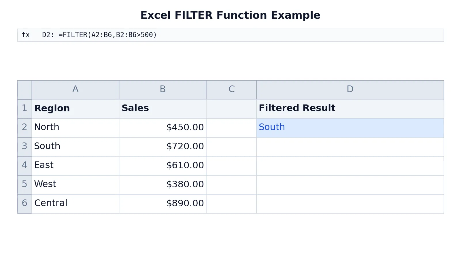
The dataset below lists five regions with their sales figures. You want to return only the rows where Sales exceed 500.

	A	B
1	Region	Sales
2	North	450
3	South	720
4	East	610
5	West	380
6	Central	890

The formula in cell D2 is:

=FILTER(A2:B6,B2:B6>500)

This returns only the rows from A2:B6 where Sales in B2:B6 is greater than 500. The first matching row is South with 720, so the spilled result begins with South and continues with the other rows that pass the test.

The include argument B2:B6>500 produces this logical array:

$$ \text{include} = \{\text{FALSE}, \text{TRUE}, \text{TRUE}, \text{FALSE}, \text{TRUE}\} $$

FILTER keeps rows 2, 3, and 5 of the array (South, East, and Central) and drops North and West. The result spills down from D2.

More Examples

Filter with a text condition. To return only the North row:

=FILTER(A2:B6,A2:A6="North")

The include array is A2:A6="North", which is TRUE only for the first row.

Filter with two conditions (AND). To return rows where Sales exceed 500 and the region is not West:

=FILTER(A2:B6,(B2:B6>500)*(A2:A6<>"West"))

Multiplying two logical arrays gives AND logic. A row is kept only when both tests are TRUE.

Filter with two conditions (OR). To return rows where Sales exceed 800 or Sales are below 400:

=FILTER(A2:B6,(B2:B6>800)+(B2:B6<400))

Adding two logical arrays gives OR logic. A row is kept when either test is TRUE.

Handle empty results. To avoid a #CALC! error when nothing matches:

=FILTER(A2:B6,B2:B6>1000,"No rows found")

Here no sales exceed 1000, so the formula returns the text "No rows found" instead of an error.

Filter a single column. To return just the Sales values above 500:

=FILTER(B2:B6,B2:B6>500)

This spills a single column of matching numbers.

If you need to count or sum the matching values instead of listing them, functions like SUMIF and SUMIFS are often a better fit. If you need to locate the position of a match, see the MATCH function.

Errors and How to Fix Them

Error	Cause	Fix
`#CALC!`	No rows match the condition and `if_empty` was omitted.	Add an `if_empty` value, or widen the condition.
`#VALUE!`	The `include` array dimensions do not match `array`.	Make sure both ranges have the same number of rows (or columns).
`#SPILL!`	The spilled range overlaps existing data.	Clear the cells below and to the right of the formula.
`#NAME?`	The function name is misspelled or the version does not support it.	Check the spelling and confirm your Excel version supports dynamic arrays.

The #SPILL! error is the most common one in practice. It means something is already sitting in the cells where the result wants to land. Delete or move that content and the formula recalculates.

Common Mistakes

Mismatched ranges. Writing =FILTER(A2:B6,B2:B10>500) fails because the include range has more rows than the array. Keep both ranges the same size.
Forgetting the spill needs empty space. Placing the formula directly above existing data triggers #SPILL!. Leave the area below and to the right clear.
Using AND/OR words instead of math. FILTER does not accept AND() or OR() across an array in the include argument. Use * for AND and + for OR.
Expecting case-sensitive text matching. Text comparisons in FILTER are not case sensitive, so "north" and "North" both match. Use a case-sensitive helper if you need exact case.
Copying the formula down. FILTER spills on its own. Copying it into every row creates overlapping spills and errors.
Ignoring empty results. Without if_empty, a no-match condition returns #CALC!, which looks like a broken formula to anyone reading the sheet.

Limitations

FILTER returns values, not references you can edit in place. The spilled cells are the output of one formula, so you cannot change a single result without changing the source data or the condition. If you delete a spilled cell, Excel blocks the action.

FILTER also depends on dynamic array support. In older versions of Excel that lack it, the function is not available and the formula returns #NAME?. The include argument must be a logical array of matching size, which makes cross-sheet or differently shaped ranges awkward. For interactive row hiding, the built-in filter feature described in how to filter in Excel may suit you better. For conditional logic that returns one value per row, the IFS function is a simpler tool.

Frequently Asked Questions

What does the Excel FILTER function do?

It returns the rows of a range that meet a condition you specify. You provide the array and a logical test, and it spills the matching rows into the cells around the formula. It is a dynamic array function, so one formula can return many rows.

How do I use the FILTER function with multiple conditions?

Combine logical arrays with math. Use multiplication for AND logic, as in (B2:B6>500)*(A2:A6<>"West"), and addition for OR logic, as in (B2:B6>800)+(B2:B6<400). Each condition must be the same size as the array you are filtering.

Why does my FILTER formula return #CALC!?

#CALC! means no rows matched your condition and you did not provide an if_empty value. Add a third argument such as "No results" to return a friendly message instead. You can also loosen the condition so at least one row passes.

Why does my FILTER formula return #SPILL!?

The result needs empty cells to expand into, and something is blocking them. Clear the cells below and to the right of the formula. If the block is far away, the spill range is larger than you expected, so check how many rows match.

Can FILTER return columns instead of rows?

Yes. If your include argument is a horizontal logical array, FILTER keeps matching columns. The same dimension rule applies, so the include array must match the width of the array you are filtering.

References

This article draws on the standard references listed under Further Reading.