XMATCH Function in Excel: Syntax and Examples

By Dr. Zubair Khalid, DVM, MS, PhD · 2026-10-03

XMATCH returns the relative position of a value inside a range or array. You give it a value to find and the range to search, and it tells you where that value sits, counting from the start of the range. It is the modern replacement for the older MATCH function, with clearer defaults and two extra search modes.

Quick Answer

XMATCH finds a value and returns its position, not the value itself.
The syntax is =XMATCH(lookup_value, lookup_array, [match_mode], [search_mode]) [1].
match_mode controls exact, approximate or wildcard matching. The default is 0, an exact match [1].
search_mode controls direction and method: first-to-last, last-to-first, or binary search on sorted data [1].
XMATCH is available in Excel for Microsoft 365, Excel 2024, Excel 2021 and Excel for the web, plus Google Sheets [1][2].

Syntax

$$=XMATCH(lookup\_value,\ lookup\_array,\ [match\_mode],\ [search\_mode])$$

Argument	Required?	Meaning
`lookup_value`	Required	The value you want to find. It can be a number, text, a logical value or a cell reference [1].
`lookup_array`	Required	The single row or column of cells, or array, to search through [1][2].
`match_mode`	Optional	How XMATCH decides a value matches. Defaults to 0 [1].
`search_mode`	Optional	The direction and method of the search. Defaults to 1 [1].

The match_mode values are:

Value	Behavior
0	Exact match. This is the default [1].
-1	Exact match, or the next smaller item if no exact match exists [1].
1	Exact match, or the next larger item if no exact match exists [1].
2	Wildcard match, where `*`, `?` and `~` have special meaning [1].

The search_mode values are:

Value	Behavior
1	Search first-to-last. This is the default [1].
-1	Search last-to-first, a reverse search [1].
2	Binary search that assumes `lookup_array` is sorted in ascending order [1].
-2	Binary search that assumes `lookup_array` is sorted in descending order [1].

How It Works

XMATCH walks through lookup_array and compares each entry against lookup_value using the rule you set in match_mode. When it finds a match, it returns the position of that entry relative to the first cell of the range. If the range is A2:A7 and the match is in A3, XMATCH returns 2, because A3 is the second cell in the range.

The default behavior is an exact match searching forward. That means =XMATCH("Gadget",A2:A7) and =XMATCH("Gadget",A2:A7,0,1) return the same result. You only need to write the optional arguments when you want something other than the default.

The reverse search mode is the feature that separates XMATCH from MATCH most clearly. With search_mode set to -1, XMATCH scans from the bottom of the range upward and returns the position of the last matching entry instead of the first. This is useful when a list contains duplicate values and you want the most recent one, such as the latest price for a product.

The approximate modes, -1 and 1, are for numeric data. With match_mode set to 1, XMATCH returns an exact match if one exists, and otherwise the next larger value. With -1, it returns the next smaller value. Unlike MATCH, these modes do not require the data to be sorted, because XMATCH checks every entry for the nearest qualifying value.

The binary search modes, 2 and -2, are a performance feature. They cut the search range in half on each pass, so they are much faster on large sorted lists. The trade-off is strict: if the data is not sorted in the direction you specified, XMATCH returns an invalid result instead of an error [1]. Use them only when you control the sort order of the data.

Worked Example

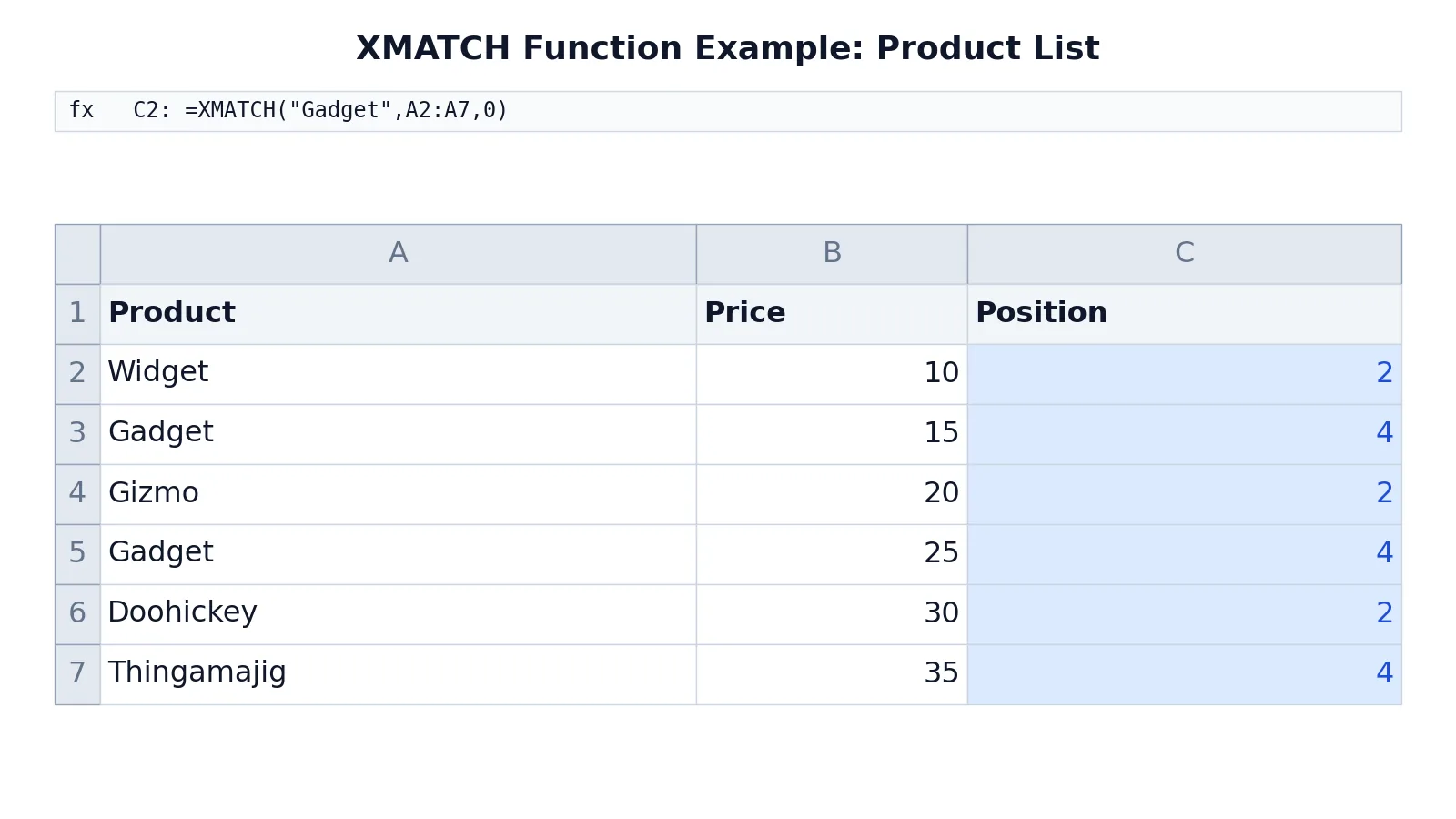
This sheet lists products in column A with prices in column B, and uses XMATCH in column C to locate the product "Gadget" under different search modes. Note that "Gadget" appears twice, in rows 3 and 5.

	A	B	C
1	Product	Price	Position
2	Widget	10	`=XMATCH("Gadget",A2:A7,0)` -> displays 2
3	Gadget	15	`=XMATCH("Gadget",A2:A7,0,-1)` -> displays 4
4	Gizmo	20	`=XMATCH("Gadget",A2:A7,0,1)` -> displays 2
5	Gadget	25	`=XMATCH("Gadget",A2:A7,0,-1)` -> displays 4
6	Doohickey	30	`=XMATCH("Gadget",A2:A7,0,1)` -> displays 2
7	Thingamajig	35	`=XMATCH("Gadget",A2:A7,0,-1)` -> displays 4

The first formula in C2 uses the default match mode and the default search mode. It finds the first "Gadget" at A3, which is position 2 in the range A2:A7.

The formula in C3 adds search_mode of -1. XMATCH now scans from the bottom of the range upward and finds the second "Gadget" at A5, which is position 4. The formulas in C4 and C6 repeat the forward search and return 2, while C5 and C7 repeat the reverse search and return 4.

The pattern is the point. The same lookup value and the same range produce 2 or 4 depending only on the search direction. If you were pulling the latest price for a product from a list that grows over time, the reverse search is the version you want.

More Examples

Return a value instead of a position. XMATCH on its own gives you a number. To get the price of the last "Gadget" entry, wrap it in INDEX:

=INDEX(B2:B7,XMATCH("Gadget",A2:A7,0,-1))  // returns 25

This combination is the standard replacement for a left-to-right lookup, and it works in any direction because INDEX takes a position and XMATCH supplies it. The same idea powers two-way lookups, where one XMATCH finds the row and another finds the column [1]. If you are used to VLOOKUP, the INDEX and XMATCH pair removes the column-counting problem entirely.

Approximate match on numbers. With match_mode set to 1, XMATCH returns an exact match or the next larger item. On the array {5,4,3,2,1}, the formula =XMATCH(4.5,{5,4,3,2,1},1) returns 1, because 5 is the next larger item and it sits first in the array [1]. With match_mode set to 0 on the same array, =XMATCH(4,{5,4,3,2,1}) returns 2, because 4 is the second entry [1].

Wildcard matching. Set match_mode to 2 and the characters *, ? and ~ take on special meaning [1]. A question mark matches one character and an asterisk matches any run of characters. This lets you find the first product code that starts with a given prefix without building a helper column.

Filtering by position. Once XMATCH gives you a position, you can feed it into other dynamic array functions. The FILTER function and SUMIF and SUMIFS both work well alongside position-based lookups when you need to return or total more than one row.

Errors and How to Fix Them

#N/A. XMATCH could not find the value. Check for trailing spaces or numbers stored as text. A case difference is not the cause, because XMATCH ignores case. Confirm the value exists in the range you passed.

#VALUE!. The lookup_array is not a single row or column. XMATCH expects a one-dimensional range, so a rectangular block will fail [2].

Wrong position from a binary search. If you used search_mode 2 or -2 on unsorted data, XMATCH returns an invalid result without warning [1]. Sort the range or switch back to search mode 1 or -1.

#SPILL! or unexpected results. This usually means the formula is part of a larger dynamic array expression and the output area is blocked. Clear the cells below and to the right of the formula.

Common Mistakes

Expecting the value back. XMATCH returns a position, not the matched item. Wrap it in INDEX or another lookup function when you need the value itself.
Assuming the default is a reverse search. The default search_mode is 1, so XMATCH returns the first match. Add -1 explicitly when you want the last one.
Using binary search on unsorted data. Modes 2 and -2 require sorted data and return invalid results silently when the sort order is wrong [1]. Verify the sort before you rely on them.
Forgetting that wildcards need match_mode 2. The * and ? characters are treated as literal text unless you set match_mode to 2 [1].
Passing a two-dimensional range. XMATCH needs a single row or column [2]. Use one XMATCH per dimension for a two-way lookup.
Confusing position with row number. A match in A3 returns 2 when the range starts at A2. The count is relative to the range, not the sheet.

Limitations

XMATCH finds one position per call. It cannot return every position where a value appears, so duplicate-heavy data needs a different approach such as FILTER or a helper column. It also does not evaluate conditions. You cannot ask it for the first product over a certain price, because it compares values for equality or proximity, not for logical tests.

The approximate and binary search modes depend on how your data is sorted, and they fail quietly when that assumption breaks. That makes them fast but fragile. For most day-to-day lookups, the exact match with a forward or reverse search is the safer choice, and the performance difference only matters on very large ranges.

Frequently Asked Questions

What is the difference between XMATCH and MATCH?

Both return the position of a value in a range. XMATCH defaults to an exact match, while MATCH defaults to an approximate match, which is a common source of wrong answers. XMATCH also adds a reverse search mode and a wildcard match mode as explicit options, and its argument order is easier to read [1].

Does XMATCH work in older versions of Excel?

No. XMATCH requires Excel for Microsoft 365, Excel 2024, Excel 2021 or Excel for the web [1]. In older versions you need MATCH or a combination of INDEX and MATCH. Google Sheets also supports XMATCH with the same core arguments [2].

How do I find the last match instead of the first?

Set the fourth argument to -1. The formula =XMATCH("Gadget",A2:A7,0,-1) searches from the bottom of the range upward and returns the position of the last matching entry [1]. This is the cleanest way to pull the most recent record from an append-only list.

Can XMATCH return the value instead of the position?

Not on its own. XMATCH always returns a number. To get the value, nest it inside INDEX, as in =INDEX(B2:B7,XMATCH("Gadget",A2:A7,0,-1)). The XMATCH supplies the row position and INDEX returns the cell at that position.

Why does XMATCH return #N/A when I can see the value?

The most common causes are trailing spaces, numbers stored as text, or hidden characters such as non-breaking spaces. Case differences do not cause it, because XMATCH ignores case. Check the cell with a function like FIND or RIGHT to inspect the actual characters, then clean the data or adjust the lookup value to match it exactly.

References

Further Reading
- Broman KW, Woo KH (2018). Data Organization in Spreadsheets. The American Statistician
- Ziemann M, Eren Y, El-Osta A (2016). Gene name errors are widespread in the scientific literature. Genome Biology
- Microsoft Support: Excel help and learning
- McCullough B, Heiser DA (2008). On the accuracy of statistical procedures in Microsoft Excel 2007. Computational Statistics & Data Analysis