What Is Data Wrangling? Definition, Steps and Examples

By Dr. Zubair Khalid, DVM, MS, PhD · 2026-10-03

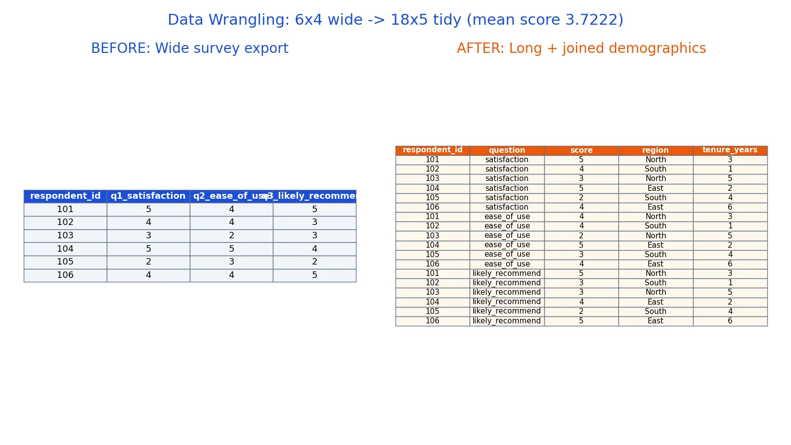
Data wrangling is the process of taking raw, awkwardly shaped data and turning it into a form you can analyze. It covers reshaping tables, joining sources, standardizing labels and fixing values that do not match. Most analysts spend more time on data wrangling than on modeling, because real datasets rarely arrive ready to use [1].

Quick Answer

Data wrangling is the broad process of getting raw data into an analyzable shape. It includes reshaping, joining, renaming, recoding and type conversion.
Data cleaning is one part of data wrangling. Cleaning fixes bad values. Wrangling also changes the structure of the data.
The usual steps are: inspect, reshape, standardize, join, validate, then document.
Wrangling produces a tidy table where each row is one observation and each column is one variable [2].
It is iterative. You often reshape, look at the result, and reshape again.

What Data Wrangling Means

In plain terms, data wrangling is everything you do between receiving data and analyzing it. You might receive three spreadsheets, a CSV export and a database dump. None of them share column names. Some store one row per person, others store one row per response. Wrangling is the work of making them agree.

The precise definition comes from the tidy data framework. A dataset is tidy when each variable forms a column, each observation forms a row, and each type of observational unit forms a table [2]. Data wrangling is the set of operations that move a dataset toward that structure. Reshaping from wide to long format is a standard example, and it comes up whenever you have repeated measures stored in separate columns [1].

The distinction from data cleaning matters. Cleaning asks "is this value correct?" Wrangling asks "is this table shaped correctly, and does it connect correctly to the other tables?" A dataset can be perfectly clean and still need heavy wrangling.

How It Works

There is no single formula for wrangling, but the mechanics reduce to a few operations. The most common is reshaping, which converts between wide and long layouts. In pandas, melt turns columns into rows and pivot does the reverse [3].

The general reshape operation can be written as a mapping from a wide table $W$ to a long table $L$:

$$L = \{(i, v, W_{iv}) : i \in \text{rows}(W),\ v \in \text{value columns}(W)\}$$

Here $i$ is the identifier column that stays fixed, $v$ is the name of a value column, and $W_{iv}$ is the cell value at that row and column. Each cell in the wide table becomes one row in the long table. If a wide table has $n$ rows and $k$ value columns, the long table has $n \times k$ rows.

The second core operation is the join, which combines two tables on a shared key:

$$J = \{ (a, b) : a \in A,\ b \in B,\ a_{\text{key}} = b_{\text{key}} \}$$

Here $A$ and $B$ are the two tables, and the key is the column they share. A left join keeps every row of $A$ and attaches matching rows from $B$, filling with missing values where no match exists.

The third operation is standardization, which is a function applied to a column:

$$s' = f(s)$$

Here $s$ is the original string or value and $f$ is the transformation, such as stripping a prefix, lowercasing text, or converting a type. You apply it column by column until the values match across sources.

Worked Example

Take a raw survey export. It has a wide table with one column per question, plus a separate demographics table with region and tenure. The wide table has 6 respondents and 4 columns: respondent_id, q1_satisfaction, q2_ease_of_use, q3_likely_recommend.

respondent_id	q1_satisfaction	q2_ease_of_use	q3_likely_recommend
101	5	4	5
102	4	4	3
103	3	2	3
104	5	5	4
105	2	3	2
106	4	4	5

The demographics table holds respondent_id, region and tenure_years for the same six people.

Step 1: Note the wide shape. The starting table is 6 rows by 4 columns. Each respondent occupies one row, and the three questions sit side by side.

Step 2: Melt to long. Reshaping gives 18 rows and 3 columns. The count is 6 respondents times 3 questions.

Step 3: Strip the question prefix. The column names q1_satisfaction, q2_ease_of_use and q3_likely_recommend become satisfaction, ease_of_use and likely_recommend. The qN_ prefix carries no information once the question is a row label.

Step 4: Join demographics. Merging on respondent_id gives 18 rows and 5 columns. Every long row picks up the region and tenure of its respondent.

Step 5: Compute the mean. The 18 scores sum to 67, so the mean is $67 / 18 = 3.7222$.

Step 6: Break it down by region. East averages 4.5000, North averages 3.6667, and South averages 3.0000.

Here is the code:

import pandas as pd
long = wide.melt(id_vars='respondent_id', var_name='question', value_name='score')
long['question'] = long['question'].str.replace(r'^q\d+_', '', regex=True)
tidy = long.merge(demo, on='respondent_id', how='left')
print(f"tidy shape = {tidy.shape}; mean score = {tidy['score'].mean():.4f}")

Output:

tidy shape = (18, 5); mean score = 3.7222

The wide table could not be averaged directly, because the three questions lived in three separate columns. After wrangling, one mean() call answers the question, and grouping by region answers the follow-up.

How to Interpret It

Read the output as a shape check first, then a value check. The shape tells you whether the wrangling worked. If you expected 18 rows and got 18, the melt is correct. If you got 24, you probably melted the respondent_id column you should have kept as an identifier.

The value check comes next. A mean of 3.7222 on a 1 to 5 scale sits above the midpoint. The regional breakdown is more interesting: East at 4.5000 is well above South at 3.0000. That gap is the kind of pattern wrangling exists to reveal. Before reshaping, you could not compute it at all.

Watch for row counts that change unexpectedly after a join. A left join should never add rows unless the right table has duplicate keys. If your row count grows, check the key column for duplicates before trusting any downstream number.

When to Use It (and when not to)

Use data wrangling whenever your source data does not match the shape your analysis needs. That covers most real work. Survey exports, web logs, database dumps and spreadsheet handoffs all arrive in shapes that need adjustment [1]. If you are combining two or more sources, you will almost certainly wrangle.

Skip heavy wrangling when the data already fits. If a table is tidy and you only need a filter and a group-by, that is analysis, not wrangling. Do not reshape for its own sake.

Also skip wrangling when the question is still unclear. Reshaping decisions depend on what you plan to compute. If you do not know whether you need one row per respondent or one row per response, you will reshape twice. Decide the analysis first, then wrangle toward it.

Data Wrangling vs Data Cleaning

These two terms overlap, and people use them interchangeably. The difference is scope. Cleaning is about the contents of cells. Wrangling is about the structure of tables and how they connect.

Aspect	Data Cleaning	Data Wrangling
Focus	Cell values	Table structure and joins
Typical tasks	Fix typos, handle missing values, correct types	Reshape, merge, rename, aggregate
Question asked	Is this value correct?	Is this table shaped right?
Scope	One column or one table	One or more tables
Order	Often inside wrangling	Often contains cleaning

In practice, cleaning is a step within wrangling. You reshape, then you notice that North and north are two different labels, then you clean them. The two activities interleave.

Common Mistakes

Melting identifier columns by accident. If you forget to list respondent_id as an id variable, it is melted like a question column and your row count grows from 18 to 24. Fix: always pass the id columns explicitly.
Joining on a non-unique key. A duplicate key in the right table multiplies your rows silently. Fix: check value_counts() on the key before merging.
Dropping rows during a join without noticing. An inner join discards unmatched rows. Fix: use a left join and count the missing values afterward.
Renaming columns before checking for collisions. Two sources may both have a column called date with different meanings. Fix: prefix columns by source, then rename deliberately.
Reshaping before deciding the analysis. You end up with a long table when you needed a wide one. Fix: sketch the target table first.
Skipping documentation. Six months later nobody remembers what q3_likely_recommend measured. Fix: keep a data dictionary alongside the wrangled output.

Limitations

Wrangling cannot fix data that was never collected. If a question was not asked, no reshape will produce it. If respondents skipped a section, the missing values stay missing, and reshaping only moves them around. Wrangling also cannot tell you whether a value is wrong. A satisfaction score of 5 looks the same whether it is genuine or a data entry error.

Reshaping changes how data looks, not what it means. A long table and a wide table contain the same information. If your conclusion changes after a reshape, the problem is in the analysis, not the shape. Treat wrangling as preparation, and keep the original raw data untouched so you can always trace back.

Frequently Asked Questions

Is data wrangling the same as data cleaning?

No, though they overlap. Cleaning fixes incorrect or inconsistent values inside cells. Wrangling covers cleaning plus reshaping, joining and restructuring tables. Most projects do both, and the two steps often alternate.

How long does data wrangling take?

It depends on the source. A single tidy CSV might take minutes. Combining several sources with different schemas can take hours or days. The work is iterative, so budget time for a second pass after you see the first result.

Do I need to know how to code to wrangle data?

No, but code helps with repeatability. Spreadsheets handle small datasets well. Once you are joining multiple sources or reshaping thousands of rows, a scripting language makes the steps reproducible and reviewable.

What is a tidy dataset?

A tidy dataset has one column per variable, one row per observation, and one table per type of observational unit [2]. Tidy structure makes downstream analysis and plotting straightforward, because most tools expect it.

Can data wrangling change my results?

It can change what you are able to compute. Reshaping a wide survey into long format is what makes a single mean possible. A join can add context that reveals patterns hidden in one table. The underlying values do not change, but the questions you can answer do.

If you want to go deeper on the surrounding concepts, see what data analysis is, data granularity, and data aggregation. For the operational side, data management basics and what a data dictionary is cover how teams keep wrangled data usable over time.