What Is Data Granularity? Definition and Examples

By Dr. Zubair Khalid, DVM, MS, PhD · 2026-10-03

Granularity definition: data granularity is the level of detail at which data is recorded, stored, or analyzed. Fine granularity keeps many small units, such as one row per day. Coarse granularity combines those units into fewer, larger groups, such as one row per month. The choice changes what questions your data can answer.

Quick Answer

Granularity is the size of the smallest unit your data describes, and it sets the floor on what analysis is possible.
Fine granularity means more rows and more detail. Coarse granularity means fewer rows and broader summaries.
Aggregation moves data from fine to coarse. It usually preserves totals but destroys within-group variation.
Granularity is relative. Daily data is fine next to monthly data and coarse next to hourly data.
The right level depends on the question. You cannot recover detail that was never captured.

What Granularity Means

In plain terms, granularity is how finely a dataset is chopped. A dataset with one row per customer is finer than one with a row per country. A dataset with one row per second is finer than one with a row per hour. The word comes from the idea of grains: smaller grains mean more pieces and more detail.

The precise statistical definition is the resolution of the unit of observation in a dataset. The unit of observation is the entity each row describes, and granularity is the specificity of that entity. A row can describe a single transaction, a single day, a single store, or a whole region. Each step up in grouping produces a coarser dataset with fewer rows.

Granularity also appears in formal work on data organization. Researchers describe hierarchies of levels that help structure and integrate data from different sources, so that comparison and analysis stay consistent across systems [1]. The same idea shows up when ontologies are aligned: mismatched levels of detail cause logical problems when classes from one system are attached to another [2]. In other words, granularity is not a cosmetic choice. It affects whether two datasets can be combined at all.

You will also see the term used outside tabular data. Emotional granularity, for example, refers to the precision with which people experience and report emotions, and that precision predicts how well they regulate them [3]. The underlying meaning is the same: how finely a concept is distinguished.

How It Works

Granularity works through grouping. You take a fine dataset and apply a grouping key, then a summary function. The grouping key defines the new unit of observation, and the summary function decides what survives.

For a count of rows, the mechanism is:

$$ n_{\text{coarse}} = \sum_{g \in G} 1 $$

where $G$ is the set of distinct groups and $n_{\text{coarse}}$ is the number of rows after grouping. For a sum, it is:

$$ S_g = \sum_{i \in g} x_i $$

where $x_i$ is the value of row $i$, $g$ is one group, and $S_g$ is the group total. The symbols mean:

$x_i$: the value in a single fine-grained row, such as one day of sales.
$g$: a group, such as one week or one month.
$S_g$: the aggregated value for that group.
$G$: the full set of groups in the dataset.

Two properties matter. First, additive measures such as counts and sums survive aggregation exactly. Second, non-additive measures such as averages, rates, and percentages do not. Averaging daily averages gives a different answer than averaging the underlying rows unless every group has the same number of rows. That is why you should aggregate raw values first and compute ratios afterward.

Worked Example

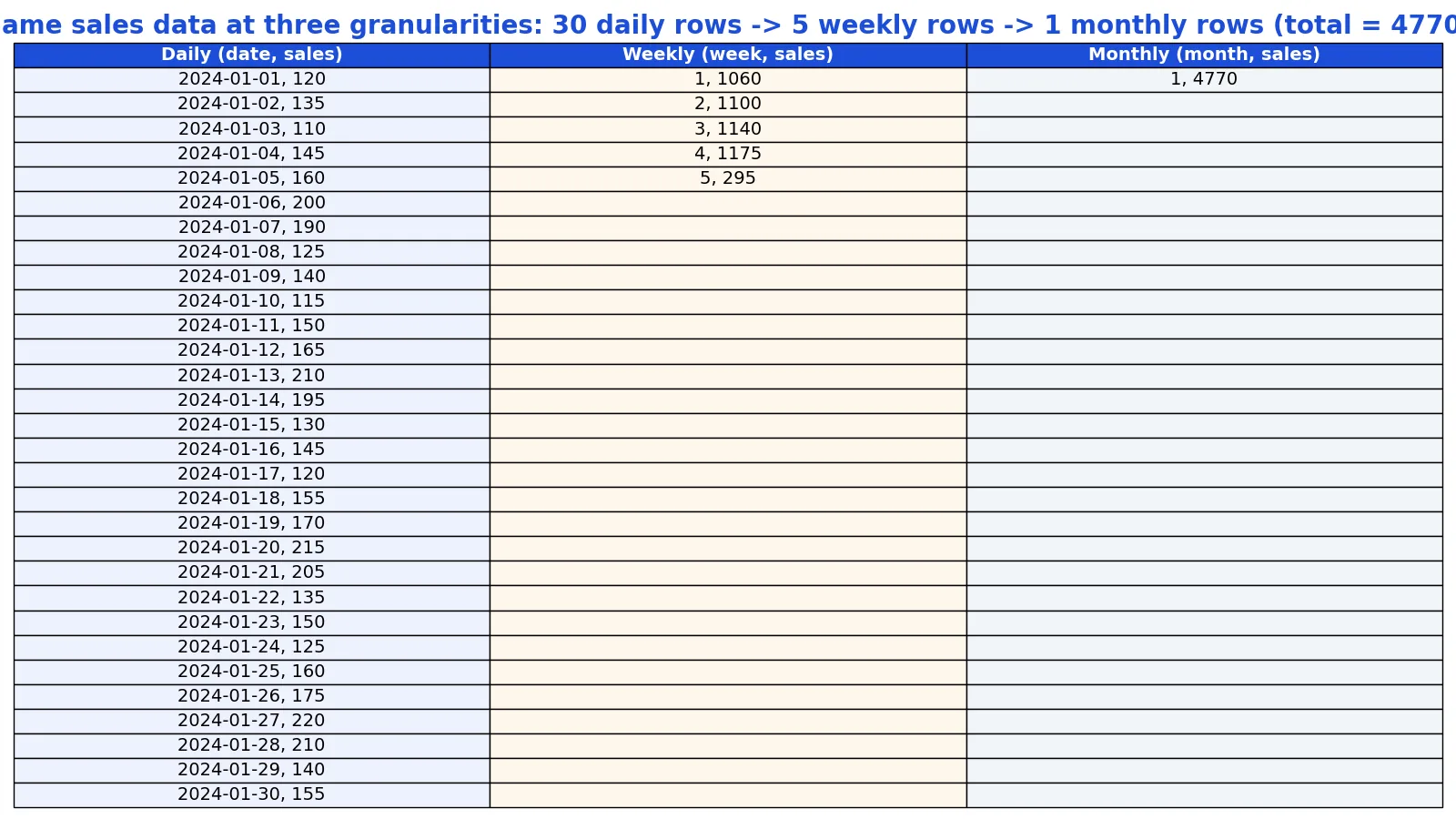
Take 30 days of daily store sales for January 2024, one row per calendar day. This is the finest granularity available in the dataset.

date	sales
2024-01-01	120
2024-01-02	135
2024-01-03	110
2024-01-04	145
2024-01-05	160
2024-01-06	200
2024-01-07	190
2024-01-08	125
2024-01-09	140
2024-01-10	115
2024-01-11	150
2024-01-12	165
2024-01-13	210
2024-01-14	195
2024-01-15	130
2024-01-16	145
2024-01-17	120
2024-01-18	155
2024-01-19	170
2024-01-20	215
2024-01-21	205
2024-01-22	135
2024-01-23	150
2024-01-24	125
2024-01-25	160
2024-01-26	175
2024-01-27	220
2024-01-28	210
2024-01-29	140
2024-01-30	155

Now walk through the aggregation steps.

Daily rows, the finest granularity: 30 rows, one per calendar day.
Weekly aggregation: grouping by week gives 5 rows. Week 1 sums to 1060.
Monthly aggregation: grouping by month gives 1 row. Month 1 sums to 4770.
Total preserved across all levels: the daily sum, the weekly sum, and the monthly sum all equal 4770.
Granularity ratio, daily to weekly to monthly: 30 : 5 : 1.

The means change with the level. The daily mean is 159, the weekly mean is 954, and the monthly mean is 4770. Those numbers are not comparable because the units differ. A daily mean describes a day, and a weekly mean describes a week.

import pandas as pd
df = pd.DataFrame({'date': pd.date_range('2024-01-01', periods=30),
                   'sales': [...]})
df['week'] = df['date'].dt.isocalendar().week
df['month'] = df['date'].dt.month
weekly = df.groupby('week')['sales'].sum()
monthly = df.groupby('month')['sales'].sum()

Output:

daily: 30 rows | weekly: 5 rows | monthly: 1 rows | total = 4770

The total is identical at every level. What you lose is the shape. The daily view shows weekend peaks on January 6, 7, 13, 14, 20, 21, 27, and 28. The monthly view shows a single number and hides every one of those peaks. This is the trade-off at the heart of granularity, and it is the same trade-off you manage when you aggregate data for reporting.

How to Interpret It

Read granularity as the resolution of your evidence. A fine dataset lets you ask narrow questions, such as which day of the week sells best. A coarse dataset lets you ask broad questions, such as whether the month beat the previous month. Neither is better in the abstract.

Check three things when you interpret a granularity choice.

First, confirm the unit of observation. If a row is a day, a count of rows is a count of days, not a count of sales. Mixing those up produces wrong conclusions.

Second, check whether the measure is additive. Sums and counts aggregate cleanly. Averages, medians, and rates need the underlying values, not the summary values.

Third, check whether the grouping key is stable. Grouping by calendar week and grouping by ISO week can produce different buckets, and that changes the numbers. The same caution applies to fiscal months and time zones.

Granularity also affects statistical tests. In enrichment analysis, changing how pathways are defined shifted p-values by up to nine orders of magnitude, while standard multiple-testing corrections typically moved them by about two orders of magnitude [4]. The lesson generalizes: the definition of your units can matter more than the statistics you run on them.

When to Use It (and when not to)

Use fine granularity when you need to detect patterns inside groups, debug anomalies, join to other fine-grained sources, or build features for a model. Fine data is also the safer default because you can always aggregate down later.

Use coarse granularity when the question is genuinely about the group, when storage or query cost is a real constraint, when you need to protect privacy by reducing identifiability, or when the fine detail is mostly noise.

Avoid aggregating early if any downstream question might need detail. Aggregation is a one-way operation in practice. Once you store monthly totals, the daily rows are gone unless you kept them. If you are still cleaning and reshaping the data, keep the finest level you have while you work through the steps of data wrangling, then aggregate at the end.

Granularity vs Cardinality

These two terms get confused because both describe the size and shape of a dataset. They measure different things.

Aspect	Granularity	Cardinality
What it measures	Level of detail in the unit of observation	Number of distinct values in a column
Example	One row per day vs one row per month	A region column with 4 distinct values
Changes when you aggregate	Yes, grouping coarsens it	Often yes, distinct counts usually drop
Main use	Deciding what questions are answerable	Deciding indexing, encoding, and join strategy
Typical question	How detailed is each row?	How many unique values are there?

A dataset can be fine-grained and low-cardinality at the same time. Thirty daily rows with a region column holding four values is exactly that case. For a fuller treatment, see what cardinality means.

Common Mistakes

Aggregating before you finish cleaning. Fix: keep the finest level until the data is correct, then aggregate once. Cleaning after aggregation means redoing the work.
Averaging averages. Fix: sum the raw values and divide by the raw count. A mean of daily means only equals the true mean when every group has the same number of rows.
Assuming totals always survive. Fix: verify. Sums and counts are additive, but distinct counts, medians, and percentiles are not, and they will not reconcile across levels.
Mixing units in one table. Fix: label the unit of observation in the column name or a metadata field, so a daily mean is never compared to a weekly mean.
Treating granularity as fixed. Fix: state the level in every chart title and report. A reader who assumes daily data when you plotted weekly totals will misread the trend.
Grouping by the wrong time key. Fix: decide up front whether weeks follow the calendar or an ISO standard, and apply the same rule everywhere.

Limitations

Granularity describes resolution, not quality. A very fine dataset can still be wrong, biased, or incomplete. Adding rows at a finer level does not fix a sampling problem, and it does not make a noisy measurement precise. Fine data also costs more to store, query, and govern, and it raises privacy risk because small units are easier to re-identify.

Aggregation is lossy in a specific way. It preserves additive totals but discards the distribution inside each group. Two months with the same total can have completely different daily patterns, and the coarse view cannot tell them apart. Granularity also interacts with definitions in ways that are hard to predict. When the underlying unit definitions change, results can shift far more than any statistical correction would suggest [4]. Treat the choice of level as an analytical decision, not a formatting one.

Frequently Asked Questions

What is granularity in simple terms?

Granularity is how detailed your data is. Fine granularity means many small units, such as one row per day or per transaction. Coarse granularity means fewer, larger units, such as one row per month or per region. Smaller units give more detail and more rows.

What does granularity mean in data analysis?

In analysis, granularity is the resolution of the unit of observation. It determines which questions you can answer. You can always combine fine data into coarse groups, but you cannot split coarse data back into fine detail. That one-way property is why analysts usually keep the finest level available.

What is the difference between fine and coarse granularity?

Fine granularity records more specific units, so it captures variation inside groups. Coarse granularity records broader units, so it summarizes and hides that variation. Daily sales data is fine. Monthly sales totals are coarse. The totals may match, but only the fine version shows which days drove them.

Does aggregation change the total?

For additive measures such as sums and counts, no. In the worked example, daily, weekly, and monthly sales all total 4770. For non-additive measures such as averages, medians, and distinct counts, yes. Those values generally do not reconcile across levels, so compute them from the raw rows.

How do I choose the right level of granularity?

Start from the question. If you need to compare days, keep daily data. If you only report monthly, monthly is enough. When in doubt, keep the finest level you can afford and aggregate for presentation. Also check whether the measure is additive before you trust a summary value.

References

- Vogt L. (2019). Levels and building blocks-toward a domain granularity framework for the life sciences. Journal of biomedical semantics
- Schulz S, Boeker M, Stenzhorn H, Niggemann J. (2009). Granularity issues in the alignment of upper ontologies. Methods of information in medicine
- "Links Between Emotion Word, Usage, Understanding, Accuracy, and Emotio" by Jennifer M.B. Fugate, Maria Gendron et al.
- Karp PD, Midford PE, Caspi R, Khodursky A. (2021). Pathway size matters: the influence of pathway granularity on over-representation (enrichment analysis) statistics. BMC genomics
Further Reading
- Wilson G, Bryan J, Cranston K et al. (2017). Good enough practices in scientific computing. PLOS Computational Biology
- Wilkinson MD, Dumontier M, Aalbersberg IJ et al. (2016). The FAIR Guiding Principles for scientific data management and stewardship. Scientific Data