Qualitative vs Quantitative Data: Types and Examples

By Dr. Zubair Khalid, DVM, MS, PhD · 2026-10-03

To decide whether your data is qualitative or quantitative, ask one question: does the value measure an amount, or does it describe a category or quality? Numbers that measure amounts are quantitative. Labels, names and ranked categories are qualitative. The phrase "data qualitative or quantitative" comes up constantly in stats courses because the answer decides which charts, averages and tests are valid.

Quick Answer

Quantitative data is numeric and measurable. You can add, subtract and average it. Examples: age, height, income, temperature.
Qualitative data is categorical or descriptive. You can count how often each category appears, but averaging the labels is meaningless. Examples: eye colour, blood type, city of birth.
Quantitative splits into discrete (countable whole steps, like number of children) and continuous (any value on a scale, like height in centimeters).
Qualitative splits into nominal (unordered labels, like eye colour) and ordinal (ordered labels, like a 1 to 5 satisfaction rating).
The type of your variable decides the right summary. Use counts and modes for nominal data, medians for ordinal data, and means with standard deviations for quantitative data.

Key Differences

Feature	Qualitative	Quantitative
What it captures	Qualities, labels, categories	Amounts, counts, measurements
Typical values	Words or codes	Numbers with units
Arithmetic allowed	No (counting categories only)	Yes (add, subtract, average)
Subtypes	Nominal, ordinal	Discrete, continuous
Central tendency	Mode, or median for ordinal	Mean, median, mode
Typical charts	Bar chart, pie chart	Histogram, box plot, scatter plot
Example from survey	eye_colour, satisfaction	age, height_cm

A useful test: if you doubled every value, would the result still make sense? Doubling a height of 171.75 cm gives 343.5 cm, which is a real (if tall) measurement. Doubling an eye colour or a satisfaction label of "4" gives nothing meaningful. That is the dividing line.

Qualitative Data Explained

Qualitative data records a quality or category. The values are names, labels or codes. You can sort them into groups and count how many fall in each group, but the labels themselves carry no numeric magnitude.

Nominal data is qualitative data with no natural order. Eye colour is the classic case. Blue, Brown, Green and Hazel have no ranking. You could assign numbers to them (Blue = 1, Brown = 2) but those numbers are just codes. The mean of those codes is meaningless.

Ordinal data is qualitative data with a meaningful order but unknown spacing between the levels. A satisfaction rating from 1 to 5 is ordinal. You know 5 is better than 4, and 4 is better than 3. You do not know that the gap between 4 and 5 equals the gap between 1 and 2. That is why the median and mode are the right summaries for ordinal data, not the mean.

For a deeper treatment of these two families, see nominal vs ordinal variables and the broader types of data: nominal, ordinal, interval, ratio. If you want more worked cases of non-numeric evidence, qualitative data examples covers how to recognize and use them.

Quantitative Data Explained

Quantitative data records an amount. The values are numbers, and the numbers behave like numbers. You can add them, average them and compare their distances.

Discrete data comes in countable steps. The number of children in a family, the number of website visits, and a person's age in whole years are all discrete. You can list the possible values (22, 23, 24 and so on) and there is nothing between them. Age in whole years is discrete even though age itself is continuous, because the recorded values jump in one-year steps.

Continuous data can take any value in a range, limited only by how precisely you measure. Height, weight, temperature and time are continuous. A height of 171.75 cm is a valid reading, and so is 171.753 cm if your instrument is good enough.

The distinction matters for how you present the data. Discrete counts are often shown as bar charts of frequencies. Continuous measurements are usually shown as histograms or box plots, where the bars represent intervals on a continuous axis. For more numeric cases, see quantitative data examples.

Worked Example

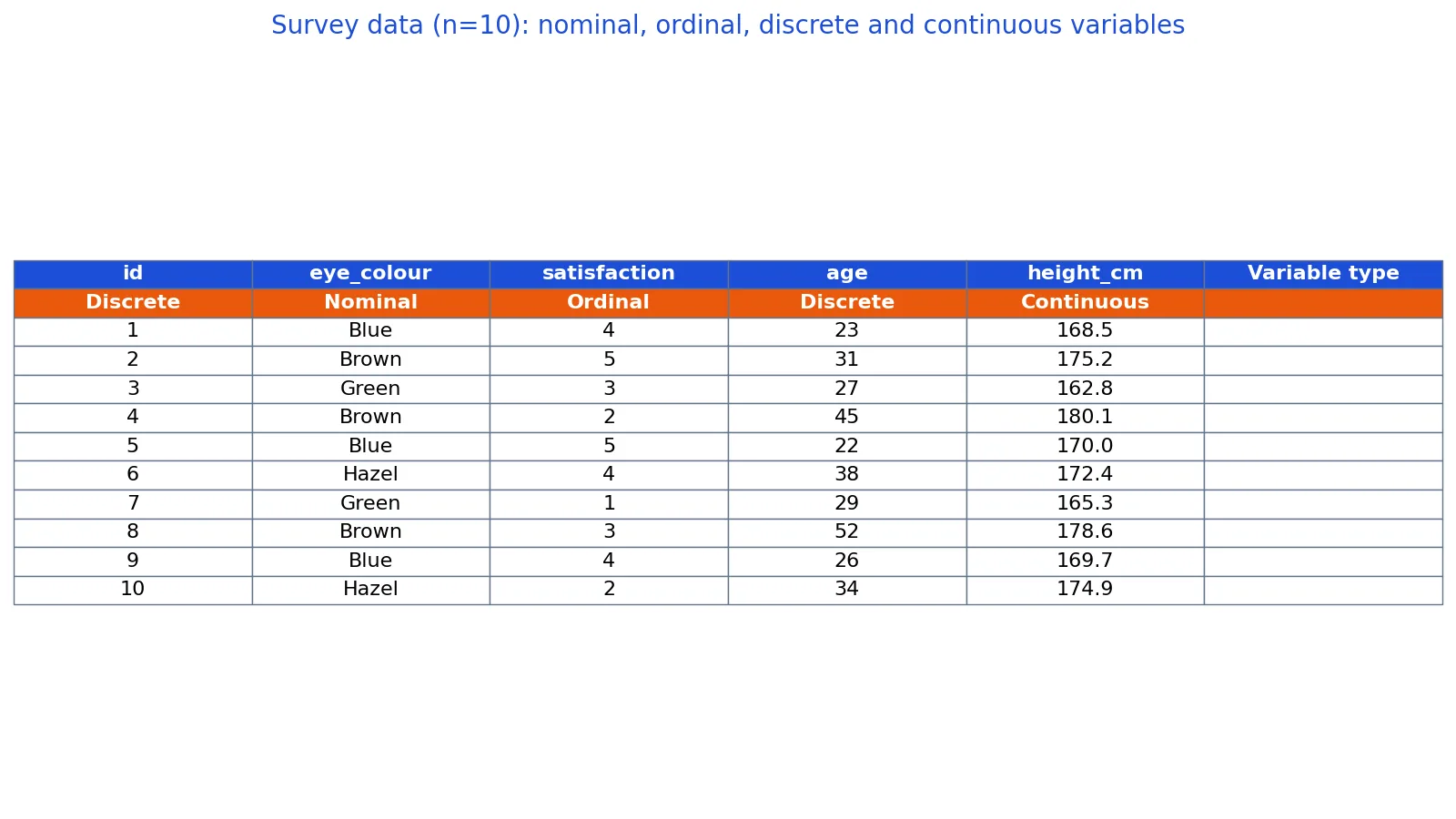
Here is a 10-row survey dataset with eye colour, satisfaction rating, age and height. Each variable has a different type, which makes it a good classification exercise.

id	eye_colour	satisfaction	age	height_cm
1	Blue	4	23	168.5
2	Brown	5	31	175.2
3	Green	3	27	162.8
4	Brown	2	45	180.1
5	Blue	5	22	170.0
6	Hazel	4	38	172.4
7	Green	1	29	165.3
8	Brown	3	52	178.6
9	Blue	4	26	169.7
10	Hazel	2	34	174.9

Step 1: Classify each column. The dataset has n = 10 rows. The id column is an identifier, a nominal label that is unique per row and not a measurement. eye_colour is nominal, with categories Blue, Brown, Green and Hazel. satisfaction is ordinal, on a 1 to 5 scale. age is discrete quantitative, with a minimum of 22 and a maximum of 52. height_cm is continuous quantitative, ranging from 162.8 to 180.1.

Step 2: Summarize the qualitative variables. For eye_colour, count the categories: Blue = 3, Brown = 3, Green = 2, Hazel = 2. For satisfaction, the median is 3.5000 and the mode is 4. The mode is the most frequent rating, and the median splits the ordered ratings in half. Reporting a mean satisfaction of 3.3 would be questionable because the spacing between rating levels is not guaranteed to be equal.

Step 3: Summarize the quantitative variables. For age, the mean is

$$\bar{x} = \frac{\sum x}{n} = \frac{327}{10} = 32.7000$$

The sample standard deviation uses n - 1 in the denominator:

$$s = \sqrt{\frac{\sum (x - \bar{x})^2}{n - 1}} = 9.7531$$

For height, the mean is 1717.5 / 10 = 171.7500 cm and the sample standard deviation is 5.5620 cm. Notice that age is discrete and height is continuous. That difference affects the chart you choose, not the arithmetic.

Step 4: Reproduce it in code. The same values come out of pandas:

import pandas as pd
df = pd.DataFrame({
    'eye_colour': ['Blue','Brown','Green','Brown','Blue','Hazel','Green','Brown','Blue','Hazel'],
    'satisfaction': [4,5,3,2,5,4,1,3,4,2],
    'age': [23,31,27,45,22,38,29,52,26,34],
    'height_cm': [168.5,175.2,162.8,180.1,170.0,172.4,165.3,178.6,169.7,174.9],
})
print(f"age std (n-1) = {df['age'].std(ddof=1):.4f}")
print(f"height std (n-1) = {df['height_cm'].std(ddof=1):.4f}")
print(f"satisfaction median = {df['satisfaction'].median()}, mode = {df['satisfaction'].mode()[0]}")

Output:

age std (n-1) = 9.7531
height std (n-1) = 5.5620
satisfaction median = 3.5, mode = 4

In Excel, with the table starting at A1 so that age sits in column D, the same age standard deviation comes from =STDEV.S(D2:D11), which returns 9.7531. If you want to see how these variables behave together, bivariate data covers pairs of variables, and correlation vs covariance explains what those joint summaries mean.

Which One Should You Use?

The choice is not really yours. The variable decides. You record what the question requires, then classify it.

Use qualitative data when the question is about categories, labels or ranked opinions. "Which eye colour is most common?" and "What is the typical satisfaction level?" are qualitative questions. Report counts, percentages, modes and medians.

Use quantitative data when the question is about amounts. "What is the average age?" and "How much does height vary?" are quantitative questions. Report means, standard deviations, ranges and percentiles.

If you have a choice at the design stage, quantitative variables give you more analytical options because they support arithmetic. But converting a genuine category into a number does not make it quantitative. A customer ID of 4021 is still a label, even though it looks like a number. For more on how data is organized before analysis, see dataset examples and structured vs unstructured data.

Common Mistakes

Averaging ordinal ratings. Computing a mean satisfaction of 3.3 treats the gap between 1 and 2 as equal to the gap between 4 and 5. Fix: report the median and mode, or state clearly that you are treating the scale as interval.
Treating ID numbers as quantitative. Averaging customer IDs or zip codes produces a number with no meaning. Fix: classify identifiers as nominal labels and use them only for grouping.
Calling whole-number measurements discrete. Height recorded to one decimal is continuous. Age recorded in whole years is discrete. Fix: check whether the underlying quantity can take intermediate values, not whether the recorded values happen to be whole.
Using a pie chart for continuous data. Pie charts show parts of a whole, which suits nominal categories. Fix: use a histogram or box plot for continuous measurements.
Assuming ordinal data is interval. A 1 to 5 scale does not guarantee equal spacing. Fix: use nonparametric methods or report medians unless you have evidence the spacing is equal.
Mixing types in one summary. Reporting a mean for eye colour and a mode for height inverts the correct treatment. Fix: classify every column first, then pick the summary that matches.

Limitations

Classification is a modeling decision, not a fact about the world. The same underlying quantity can be recorded as discrete or continuous depending on precision. Age is continuous in reality but discrete when you record whole years. Income is continuous in theory but often reported in bands, which turns it into ordinal data. Your analysis inherits the limitations of how the data was recorded.

The nominal and ordinal split also depends on context. A satisfaction scale is ordinal by default, but many analysts treat it as interval when the scale is well designed and the analysis needs a mean. That is a judgment call, and it should be stated openly. When in doubt, report the median alongside the mean so readers can see whether the choice changes the story.

Frequently Asked Questions

Is age qualitative or quantitative?

Age is quantitative because it measures an amount of time. Recorded in whole years it is discrete, since the values step in one-year increments. Recorded with decimals it is continuous. Either way, you can average it and compute a standard deviation.

Can qualitative data be turned into numbers?

You can assign numeric codes to categories, and you can count how many observations fall in each category. Those counts are quantitative. The codes themselves remain labels, so averaging them is usually meaningless unless the categories have a genuine order and equal spacing.

What is the difference between discrete and continuous data?

Discrete data has countable steps with nothing in between, like the number of children in a family. Continuous data can take any value in a range, limited only by measurement precision, like height or temperature. A quick test: can the value be split into smaller meaningful units? If yes, it is continuous.

Is a Likert scale qualitative or quantitative?

A Likert scale is ordinal, which is a type of qualitative data. The response options have a clear order but the spacing between them is not guaranteed to be equal. Report the median and mode, or justify treating the scale as interval before reporting a mean.

How do I decide the type of a variable quickly?

Ask two questions in order. First, does the value measure an amount? If yes, it is quantitative, then check whether it is countable or continuous. If no, it is qualitative, then check whether the categories have a natural order. That gives you one of four types: nominal, ordinal, discrete or continuous.

References

This article draws on the standard references listed under Further Reading.