How to Shade Every Other Row in Excel (Banded Rows)

By Dr. Zubair Khalid, DVM, MS, PhD · 2026-10-03

If you want to know how do I shade every other row in Excel, you have two reliable options. Convert your range to an Excel Table and pick a banded row style, or select the range and apply a conditional formatting rule with the formula =MOD(ROW(),2)=0. The table route updates automatically as you add rows, while the formula route works on any range and gives you full control over the fill color.

Quick Answer

Fastest method: select your data, press Ctrl+T, confirm the range, then pick a style with banded rows in Table Design.
Most flexible method: select the range, open Home > Conditional Formatting > New Rule > Use a formula to determine which cells to format, and enter =MOD(ROW(),2)=0.
The formula logic: ROW() returns the current row number, MOD(ROW(),2) returns 0 for even rows and 1 for odd rows, so =MOD(ROW(),2)=0 shades even rows.
To shade odd rows instead: use =MOD(ROW(),2)=1.
To keep the pattern aligned to your data: subtract the header row, for example =MOD(ROW()-1,2)=0 when row 1 is a header.

Before You Start

Decide what you are shading. If you only need visual separation for a static list, conditional formatting on the range is enough. If the data will grow, shrink, or feed formulas and charts, an Excel Table is the better container because the banding is part of the style and new rows inherit it.

Check three things before you apply anything.

First, confirm where your data starts. If row 1 holds headers and data begins in row 2, a plain =MOD(ROW(),2)=0 rule shades row 2, row 4, and so on. That usually looks correct because the first data row is shaded. If your data starts in row 3 or later, the pattern can look offset, and you fix it by subtracting the first data row number.

Second, select the full width you want banded. Conditional formatting applies to the selected cells only. If you select A1:C11 but your table extends to column F, columns D through F stay unshaded.

Third, clear any existing fills. Manual fill colors sit underneath conditional formatting and can make the result look patchy. Select the range, then use Home > Clear > Clear Formats if you want a clean slate.

If you are still arranging the sheet, it helps to have your rows in order first. Adding or removing rows later is easier once the banding rule is in place, and the steps for adding multiple rows in Excel work fine on a banded range.

Step by Step

These are the interface steps for the conditional formatting method.

Select the range you want to shade, for example A1:C11.
Go to Home > Conditional Formatting > New Rule > Use a formula to determine which cells to format.
Enter =MOD(ROW(),2)=0 in the formula box.
Click Format, choose a light fill color on the Fill tab, then click OK.
Click OK again to apply the rule.

The rule now shades every even-numbered row in the selection. Because the formula uses ROW() without a cell reference, it evaluates per row and the pattern repeats down the whole range.

For the table method, the steps are shorter.

Select any cell inside your data.
Press Ctrl+T and confirm the range and the "My table has headers" setting.
On the Table Design tab, choose a table style that includes banded rows.
If banding is off, check the Banded Rows box on the Table Design tab.

The table style applies banding across the full table width automatically, and the pattern continues when you type in the row directly below the table.

Worked Example

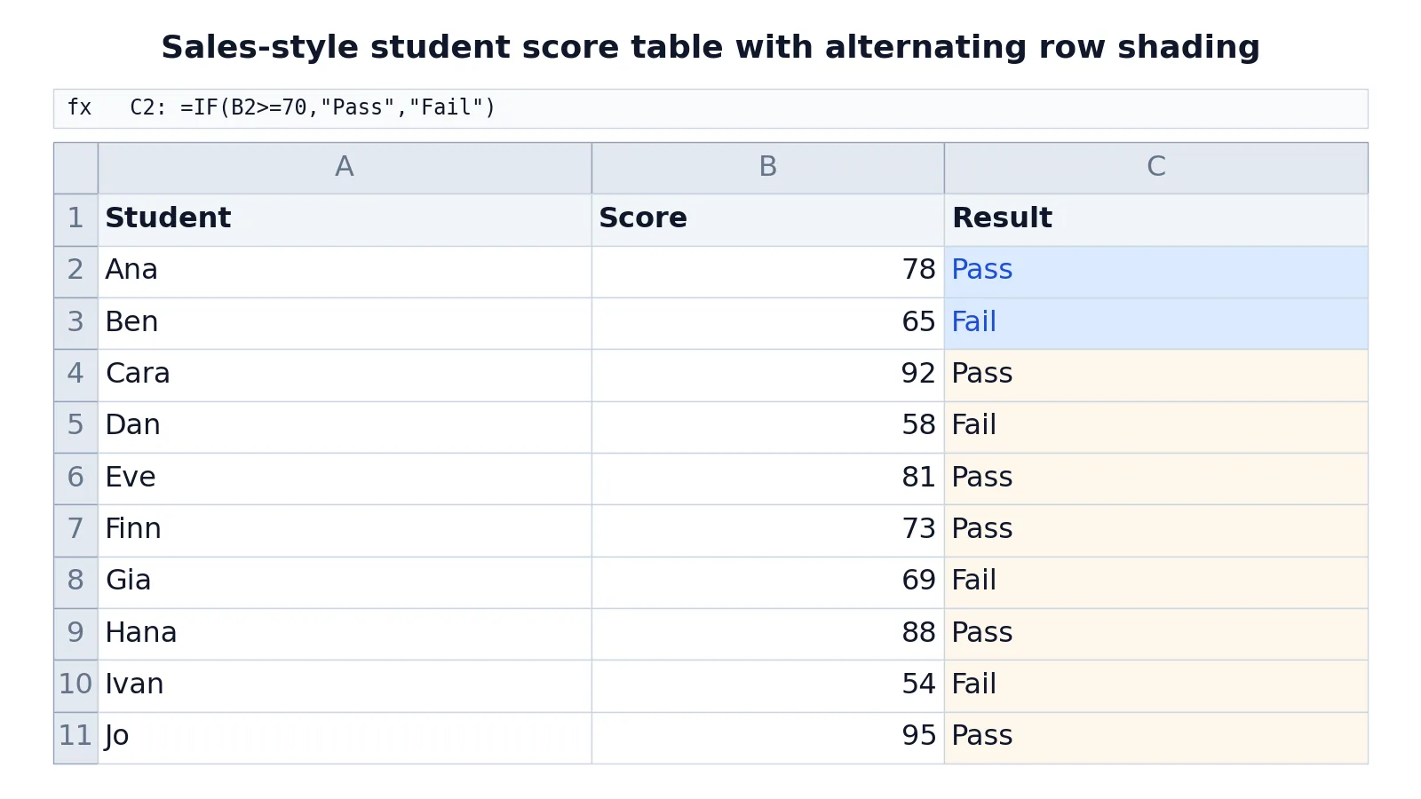
Take a small score table with 10 students. Column A holds the name, column B holds the score, and column C holds a pass or fail result computed with an IF formula.

	A	B	C
1	Student	Score	Result
2	Ana	78	`=IF(B2>=70,"Pass","Fail")` -> displays Pass
3	Ben	65	`=IF(B3>=70,"Pass","Fail")` -> displays Fail
4	Cara	92	`=IF(B4>=70,"Pass","Fail")` -> displays Pass
5	Dan	58	`=IF(B5>=70,"Pass","Fail")` -> displays Fail
6	Eve	81	`=IF(B6>=70,"Pass","Fail")` -> displays Pass
7	Finn	73	`=IF(B7>=70,"Pass","Fail")` -> displays Pass
8	Gia	69	`=IF(B8>=70,"Pass","Fail")` -> displays Fail
9	Hana	88	`=IF(B9>=70,"Pass","Fail")` -> displays Pass
10	Ivan	54	`=IF(B10>=70,"Pass","Fail")` -> displays Fail
11	Jo	95	`=IF(B11>=70,"Pass","Fail")` -> displays Pass

The formula in C2 returns Pass when the score is at least 70, otherwise Fail. The same rule filled down to the next row adjusts the row reference, so C3 reads =IF(B3>=70,"Pass","Fail") and returns Fail.

Now apply banding to A1:C11 with the rule =MOD(ROW(),2)=0. Rows 2, 4, 6, 8, and 10 get the fill. Rows 3, 5, 7, 9, and 11 stay white. The header in row 1 also stays unshaded because 1 is odd.

The pattern is easy to verify. Row 2 holds Ana with a score of 78 and a Pass result, and that row is shaded. Row 3 holds Ben with 65 and a Fail result, and that row is not shaded. The shading does not depend on the values in the cells, only on the row number, so the alternating pattern stays intact no matter how the scores change.

If you later chart this data, the banding does not travel with the chart. Alternating fills are a reading aid for the grid, and gridlines and tick marks serve a similar purpose in plots [1]. For a visual of the same data, see how to make a chart in Excel.

Other Ways to Do It

Table styles. Converting to a table gives you banded rows as a built-in style option. You can switch styles at any time on the Table Design tab, and the banding follows the table as it grows. This is the cleanest option when the data is a real dataset you will keep updating.

Manual fill. You can select a row, pick a fill color, then copy that row's format to other rows with the Format Painter. This works for a one-off printout but breaks the moment you insert or delete rows, because the fills do not move with the data.

Alternate row color via a helper column. If you need the banding to respond to something other than the row number, such as grouping by a category, add a helper column and base the rule on that column instead. For example, a rule like =MOD($D2,2)=0 shades rows based on the value in D rather than the physical row.

Group-based banding. When you want a new color block each time a value changes, a formula that compares the current row to the row above can do it. This is a different pattern from simple alternating rows, and it is useful for grouped reports.

If your sheet is long and you want the header to stay visible while you scroll through banded rows, freezing rows and columns pairs well with banding.

Troubleshooting

The pattern starts on the wrong row. Your data probably does not start in row 1 or row 2. Adjust the formula so the first data row evaluates to 0. If data starts in row 3, use =MOD(ROW()-1,2)=0.

Nothing happens after you click OK. Check that the rule is a formula rule and not a cell value rule. The formula box only appears under "Use a formula to determine which cells to format."

Only part of the row is shaded. Your selection did not cover the full width. Reselect the full range and reapply the rule, or edit the rule's "Applies to" range in Conditional Formatting > Manage Rules.

The banding disappears when you sort or filter. Conditional formatting based on ROW() follows the physical row, so sorting moves values between shaded and unshaded rows. Table banding behaves the same way because it is also tied to row position. If you need the color tied to a record, base the rule on a column value instead.

The fill looks uneven or dirty. Manual fills are showing through. Clear formats on the range, then reapply the conditional rule.

New rows below the range are not shaded. Conditional formatting only covers the range you selected. Extend the "Applies to" range, or switch to a table so new rows inherit the style.

Common Mistakes

Using =MOD(ROW(),2)=0 on a range that starts below row 2 without adjusting. The pattern looks offset. Fix it by subtracting the first data row number, for example =MOD(ROW()-3,2)=0 when data starts in row 3.
Selecting a single column instead of the full table width. Only that column gets banded. Fix it by reselecting all columns before applying the rule.
Leaving manual fills in place. The conditional fill and the manual fill fight each other. Fix it by clearing formats first.
Assuming banding survives sorting as a record attribute. It does not, because the rule keys off row position. Fix it by keying the rule off a column value if the color must follow a record.
Applying the rule to an entire column. This can slow a large workbook and shades rows far below your data. Fix it by limiting the range to the used rows.
Forgetting that the header row counts. A header in row 1 shifts which rows are even. Fix it by testing the rule on a few rows and adjusting the offset.

Limitations

Banded rows are a reading aid, not a data feature. The shading carries no meaning, so it cannot encode a category, a threshold, or a ranking. If you need color to mean something, use a rule that tests a value, such as highlighting scores below a cutoff, which is closer to what highlighting duplicates in Excel does with repeated values.

Conditional formatting also adds calculation work. A rule applied to a very large range recalculates as the sheet changes, and many rules on one sheet can slow editing. Table banding is lighter because it is a style, but it still applies to the whole table. On very wide sheets, banding every other row can compete visually with borders and gridlines, so keep the fill light and consistent.

Frequently Asked Questions

How do I shade every other row in Excel without a table?

Select the range, then use Home > Conditional Formatting > New Rule > Use a formula to determine which cells to format and enter =MOD(ROW(),2)=0. Choose a light fill and click OK. This shades even rows in the selection and works on any range, table or not.

How do I shade every third row instead of every other row?

Change the divisor in the MOD formula. Use =MOD(ROW(),3)=0 to shade every third row, or =MOD(ROW(),3)=1 to shift which row in each group of three gets the fill. The same offset trick applies if your data does not start in row 1.

Why does my banding shift when I sort the data?

The rule keys off the physical row number, so after a sort the values move but the shaded rows stay where they are. If the color needs to follow a specific record, base the rule on a column value, for example =MOD($D2,2)=0, instead of ROW().

Can I shade every other row based on a cell value?

Yes. Replace ROW() with a reference to the column that drives the pattern. A rule like =MOD($B2,2)=0 shades rows where the value in column B is even, which is useful when the banding should reflect the data rather than the row position.

Does banded row shading work in Excel tables and PivotTables?

Excel Tables support banded rows as a built-in style option on the Table Design tab. PivotTables have their own banded row and banded column style options under PivotTable Design, and those follow the pivot layout rather than the worksheet row numbers.

References

Krzywinski M (2013). Axes, ticks and grids. Nature Methods

References

Further Reading
- Broman KW, Woo KH (2018). Data Organization in Spreadsheets. The American Statistician
- Ziemann M, Eren Y, El-Osta A (2016). Gene name errors are widespread in the scientific literature. Genome Biology
- Microsoft Support: Excel help and learning
- McCullough B, Heiser DA (2008). On the accuracy of statistical procedures in Microsoft Excel 2007. Computational Statistics & Data Analysis
- Abeysooriya M, Soria M, Kasu MS et al. (2021). Gene name errors: Lessons not learned. PLOS Computational Biology