How to Add Multiple Rows in Excel (Step by Step)
By Dr. Zubair Khalid, DVM, MS, PhD ·
To add multiple rows in Excel, you write a SUM formula that references a range of cells, such as =SUM(B2:B13). That single formula adds every value in the range, and it updates automatically when you insert or delete rows inside it [1]. This guide shows how to addition multiple rows in Excel with AutoSum, manual ranges, and a conditional version that totals only the rows that pass a test.
Quick Answer
- Type
=SUM(then select the cells you want to add, or type the range directly, for example=SUM(B2:B13). - Press Enter. The formula returns the total of every numeric cell in the range.
- For a fast total, select the cell below your numbers and use Home > AutoSum, which inserts a SUM formula for you.
- SUM ignores text values in the range, so a stray label will not cause a #VALUE! error the way
=A1+B1+C1can [1]. - To total only some rows, wrap the range in a condition, for example
=SUMIF(C2:C13,"Yes",B2:B13).
Before You Start
Check three things before you build the formula.
First, make sure your numbers are real numbers. Values that look numeric but are stored as text will be skipped by SUM, and your total will be too low. You can spot them because they usually sit left-aligned in the cell while true numbers sit right-aligned.
Second, decide whether you want a total of all rows or a total of selected rows. A plain SUM range adds everything. A conditional total adds only the rows that meet a rule, which is what you want when you are totaling a subset such as sales above a target.
Third, leave the total row outside the range you are summing. If your data runs from row 2 to row 13, put the total in row 14. If you include the total cell inside its own range, you create a circular reference and Excel will warn you.
If your sheet has blank rows mixed into the data, clean those up first so your ranges stay predictable. The steps in how to delete blank rows in Excel cover that cleanup.
Step by Step
- Click the cell where you want the total to appear. For a column of numbers, this is usually the first empty cell below the last value.
- Type
=SUM(to start the formula. - Select the range with your mouse, or type it. Dragging from the first value to the last value produces something like
B2:B13. - Type
)to close the formula and press Enter. The cell now shows the total. - To use AutoSum instead, select the total cell, go to Home > AutoSum, and Excel inserts a SUM formula for the range it detects above or to the left. Press Enter to accept it.
- To total only rows that meet a condition, use SUMIF or SUM with IF. For example,
=SUMIF(C2:C13,"Yes",B2:B13)adds the values in B2:B13 only where the matching cell in C2:C13 equals "Yes".
The AutoSum route is the fastest for a single column. The manual range route gives you full control over exactly which rows are included.
Worked Example
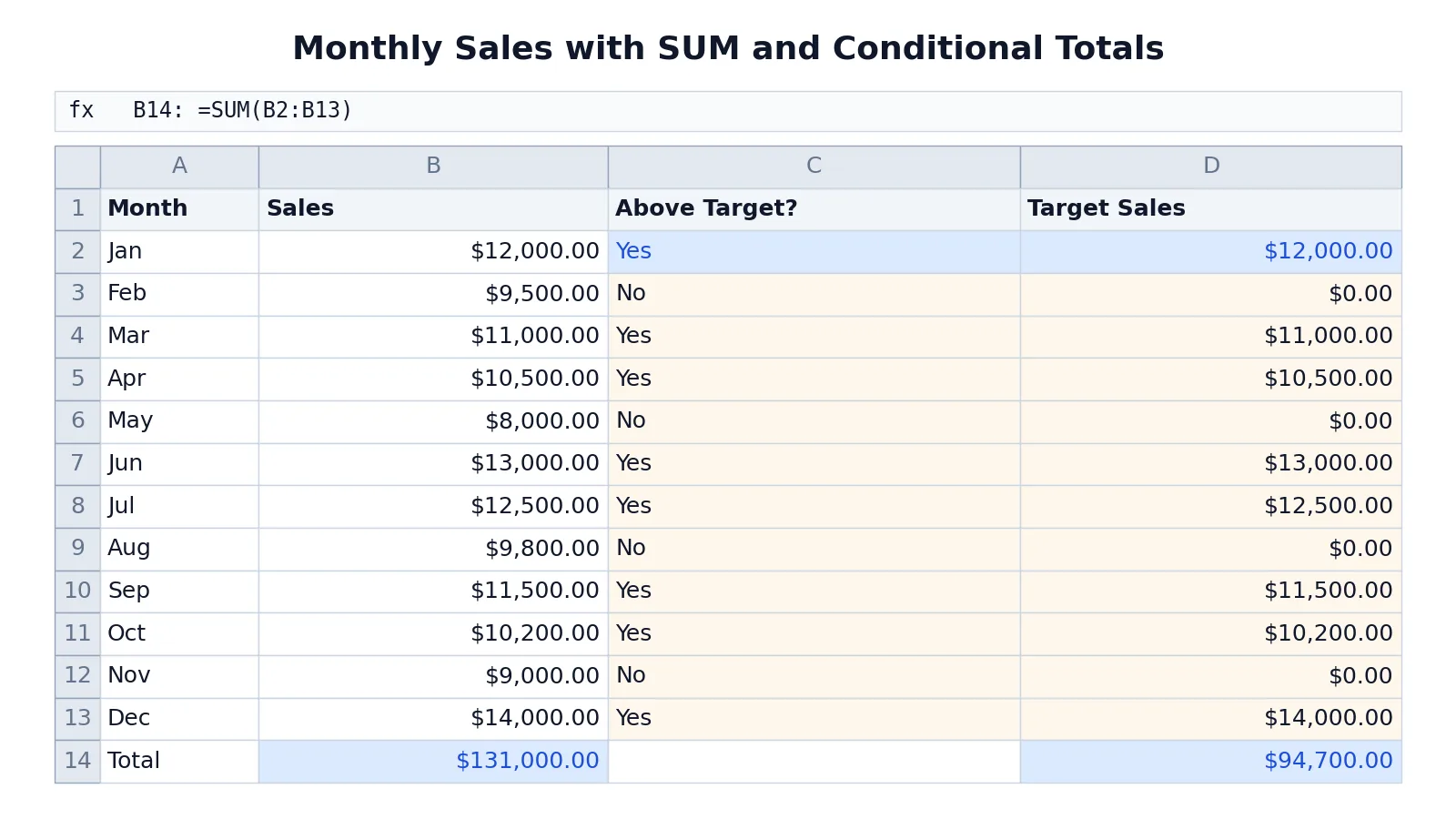
The table below is a 12-month sales sheet with a target check. Column B holds monthly sales, column C flags whether the month beat a 10,000 target, and column D returns the sales value only for months above target. The formulas are shown in the cells, and the value each one returns is listed after the arrow.
| Row | A | B | C | D |
|---|---|---|---|---|
| 1 | Month | Sales | Above Target? | Target Sales |
| 2 | Jan | 12000 | =IF(B2>10000,"Yes","No") -> Yes | =IF(C2="Yes",B2,0) -> $12,000.00 |
| 3 | Feb | 9500 | =IF(B3>10000,"Yes","No") -> No | =IF(C3="Yes",B3,0) -> $0.00 |
| 4 | Mar | 11000 | =IF(B4>10000,"Yes","No") -> Yes | =IF(C4="Yes",B4,0) -> $11,000.00 |
| 5 | Apr | 10500 | =IF(B5>10000,"Yes","No") -> Yes | =IF(C5="Yes",B5,0) -> $10,500.00 |
| 6 | May | 8000 | =IF(B6>10000,"Yes","No") -> No | =IF(C6="Yes",B6,0) -> $0.00 |
| 7 | Jun | 13000 | =IF(B7>10000,"Yes","No") -> Yes | =IF(C7="Yes",B7,0) -> $13,000.00 |
| 8 | Jul | 12500 | =IF(B8>10000,"Yes","No") -> Yes | =IF(C8="Yes",B8,0) -> $12,500.00 |
| 9 | Aug | 9800 | =IF(B9>10000,"Yes","No") -> No | =IF(C9="Yes",B9,0) -> $0.00 |
| 10 | Sep | 11500 | =IF(B10>10000,"Yes","No") -> Yes | =IF(C10="Yes",B10,0) -> $11,500.00 |
| 11 | Oct | 10200 | =IF(B11>10000,"Yes","No") -> Yes | =IF(C11="Yes",B11,0) -> $10,200.00 |
| 12 | Nov | 9000 | =IF(B12>10000,"Yes","No") -> No | =IF(C12="Yes",B12,0) -> $0.00 |
| 13 | Dec | 14000 | =IF(B13>10000,"Yes","No") -> Yes | =IF(C13="Yes",B13,0) -> $14,000.00 |
| 14 | Total | =SUM(B2:B13) -> $131,000.00 | =SUM(D2:D13) -> $94,700.00 |
The first formula checks whether January sales exceed the 10,000 target and returns Yes or No. The second returns January sales if the month is above target, otherwise 0. The total in B14 sums all monthly sales to get the yearly figure. The total in D14 sums only the sales from months that are above target.
To build the two totals, select B14 and go to Home > AutoSum to insert =SUM(B2:B13). Then select D14 and go to Home > AutoSum to insert =SUM(D2:D13).
The two totals tell different stories. All twelve months add up to $131,000.00. The eight months that beat the target add up to $94,700.00. That gap is the point of the conditional column. If you only ever sum column B, you never see how much of the year came from strong months.
Other Ways to Do It
AutoSum is the quickest option for one column. Select the cell below your data and use Home > AutoSum, then press Enter.
SUMIF handles one condition. The syntax is =SUMIF(range, criteria, sum_range), where range is the cells you test, criteria is the rule, and sum_range is the cells you add.
SUMIFS handles more than one condition. The syntax is =SUMIFS(sum_range, criteria_range1, criteria1, criteria_range2, criteria2). Note that the sum range comes first here, which is the opposite order from SUMIF.
SUBTOTAL totals only the rows that are currently visible when you use function number 109, as in =SUBTOTAL(109,B2:B13). Function number 9 skips rows hidden by a filter but still counts rows you hid manually. That matters when you filter a list and want the total to reflect the filtered view. If you filter often, this is the function to reach for.
For a quick check without writing a formula, select the cells and look at the status bar at the bottom of the window. Excel shows the sum of the selection there. It is a read-only figure, so it will not stay in the sheet.
If you are summing a single column rather than several rows, the same logic applies and the steps in how to sum a column in Excel walk through it.
Troubleshooting
The total is lower than you expect. Some cells in the range hold text that looks like numbers. SUM ignores text, so those values drop out [1]. Convert them to real numbers and the total corrects itself.
You see #VALUE!. This happens when a formula references text instead of numbers, which is common with the =A1+B1+C1 style of adding cells one by one [1]. Switching to SUM fixes it because SUM skips text values.
You see #REF!. A referenced row or column was deleted. A formula that lists individual cells does not update when rows are deleted, so it breaks and returns #REF!, while a SUM range updates on its own [1].
The total did not grow after you inserted a row. A formula built from individual cell references will not update to include a newly inserted row, but a SUM range will, as long as the new row falls inside the referenced range [1]. This is the main reason to sum a range instead of listing cells.
The total includes the total cell. You dragged the range one row too far. Shrink the range so it stops at the last data row.
Common Mistakes
- Adding cells one at a time. Writing
=B2+B3+B4+...is error prone and breaks when rows change. Use=SUM(B2:B13)so the range updates automatically [1]. - Including the total row in the range. This creates a circular reference. Keep the total cell outside the summed range.
- Assuming SUM catches text numbers. It does not. Check alignment and convert text values before you trust the total.
- Using SUMIF argument order for SUMIFS. SUMIF puts the criteria range first, SUMIFS puts the sum range first. Mixing them up returns wrong results or an error.
- Forgetting that hidden rows still count. SUM adds hidden rows. Use
SUBTOTAL(109, range)if you want filtered or hidden rows excluded. - Hardcoding a number into the formula. Typing a fixed value instead of a cell reference means the total will not change when the data does.
Limitations
SUM and its conditional variants only add numeric values. They cannot combine text, and they cannot tell you why a total changed. If a value is stored as text, SUM silently skips it, which produces a total that looks plausible but is wrong. Always spot-check a few rows against the total when the stakes are high.
Conditional totals depend on the condition column being correct. In the worked example, the target total of $94,700.00 is only meaningful if the Yes and No flags in column C are right. A wrong flag quietly moves a month in or out of the total. If you build these flags with formulas, verify a couple of them by hand before you rely on the result.
Frequently Asked Questions
How do I add multiple rows in Excel with one formula?
Type =SUM( and then select the range of cells you want to add, or type the range directly such as =SUM(B2:B13). Press Enter and the formula returns the total of every numeric cell in that range. One formula replaces a long chain of individual cell references.
What is the difference between SUM and AutoSum?
They produce the same result. AutoSum is a button on the Home tab that inserts a SUM formula for you, guessing the range from the surrounding data. SUM is the function itself, which you can type and edit by hand when you need a specific range.
Why is my SUM total wrong?
The most common cause is numbers stored as text, which SUM ignores. Another cause is a range that stops short of the last row or extends into the total cell. Check the range in the formula bar and confirm the cells you expect are included.
Can I sum only the rows that meet a condition?
Yes. Use SUMIF for one condition, for example =SUMIF(C2:C13,"Yes",B2:B13), or SUMIFS for several conditions. The conditional total adds only the rows that pass your test, which is useful for totals by category, region, or status.
Does SUM update when I insert or delete rows?
A SUM range updates automatically when you insert or delete rows inside the referenced range. A formula that lists individual cells does not update, and deleting a referenced row can return a #REF! error [1]. This is why summing a range is the safer habit.
References
Further Reading
- Broman KW, Woo KH (2018). Data Organization in Spreadsheets. The American Statistician
- Ziemann M, Eren Y, El-Osta A (2016). Gene name errors are widespread in the scientific literature. Genome Biology
- Microsoft Support: Excel help and learning
- McCullough B, Heiser DA (2008). On the accuracy of statistical procedures in Microsoft Excel 2007. Computational Statistics & Data Analysis
- Abeysooriya M, Soria M, Kasu MS et al. (2021). Gene name errors: Lessons not learned. PLOS Computational Biology