How to Unhide Rows in Excel (Step by Step)

By Dr. Zubair Khalid, DVM, MS, PhD · 2026-10-03

Hidden rows in Excel leave a double line between the row headers, and you can bring them back in seconds. The fastest general method for how to unhide all rows in Excel is to click the Select All button, open the Format menu on the Home tab, and choose Unhide Rows. This guide covers that method, the row-specific method, and what to do when rows refuse to reappear.

Quick Answer

Click the Select All button, the small triangle where row 1 and column A meet, to select the whole sheet.
On the Home tab, in the Cells group, click Format.
Point to Hide & Unhide, then click Unhide Rows.
To unhide specific rows, select the row headers on both sides of the hidden ones, right-click, and choose Unhide [1].
A double line between row headers is the visual sign that a row is hidden [1].

Before You Start

Hidden rows are not deleted rows. The data is still there, formulas still reference it, and charts still plot it. Hiding only changes what you see on screen and what prints. In Excel for the web, hidden rows and columns are not printed at all, so you have to unhide them before printing if you want them in the output [2].

Two things are worth checking before you start. First, confirm that rows are actually hidden. Look at the row numbers down the left edge. If the sequence jumps, for example from 3 straight to 7, rows 4, 5, and 6 are hidden. A double line between the headers confirms it [1]. Second, check whether the sheet is protected. If row headers will not respond to right-clicks or the Unhide option is grayed out, protection is the likely cause, and you will need the password or the sheet unprotected first.

If you are working with a large sheet where rows and columns are both hidden, the same Select All approach handles both. The companion guide on how to unhide columns in Excel covers the column side in detail.

Step by Step

These are the interface steps for revealing every hidden row on a worksheet.

Click the Select All button. It is the small triangle at the top-left corner of the sheet, in the square where row 1 and column A meet. Clicking it selects every cell on the worksheet.
On the Home tab, in the Cells group, click Format.
Point to Hide & Unhide, then click Unhide Rows.

Every hidden row on that sheet becomes visible at once. If nothing happens, the rows were not hidden, or the sheet is protected.

To unhide a specific block of rows instead of the whole sheet, select the row headers immediately above and below the hidden rows. For example, if rows 4 through 6 are hidden, select row headers 3 and 7 by dragging across them. Right-click the selection and choose Unhide [1]. You can also double-click the double line between the two visible rows where the hidden rows sit [1].

One detail that trips people up: when you select adjacent rows for this purpose, the selection must include the headers of the rows on both sides of the gap. Selecting only the visible rows above the gap does nothing.

Worked Example

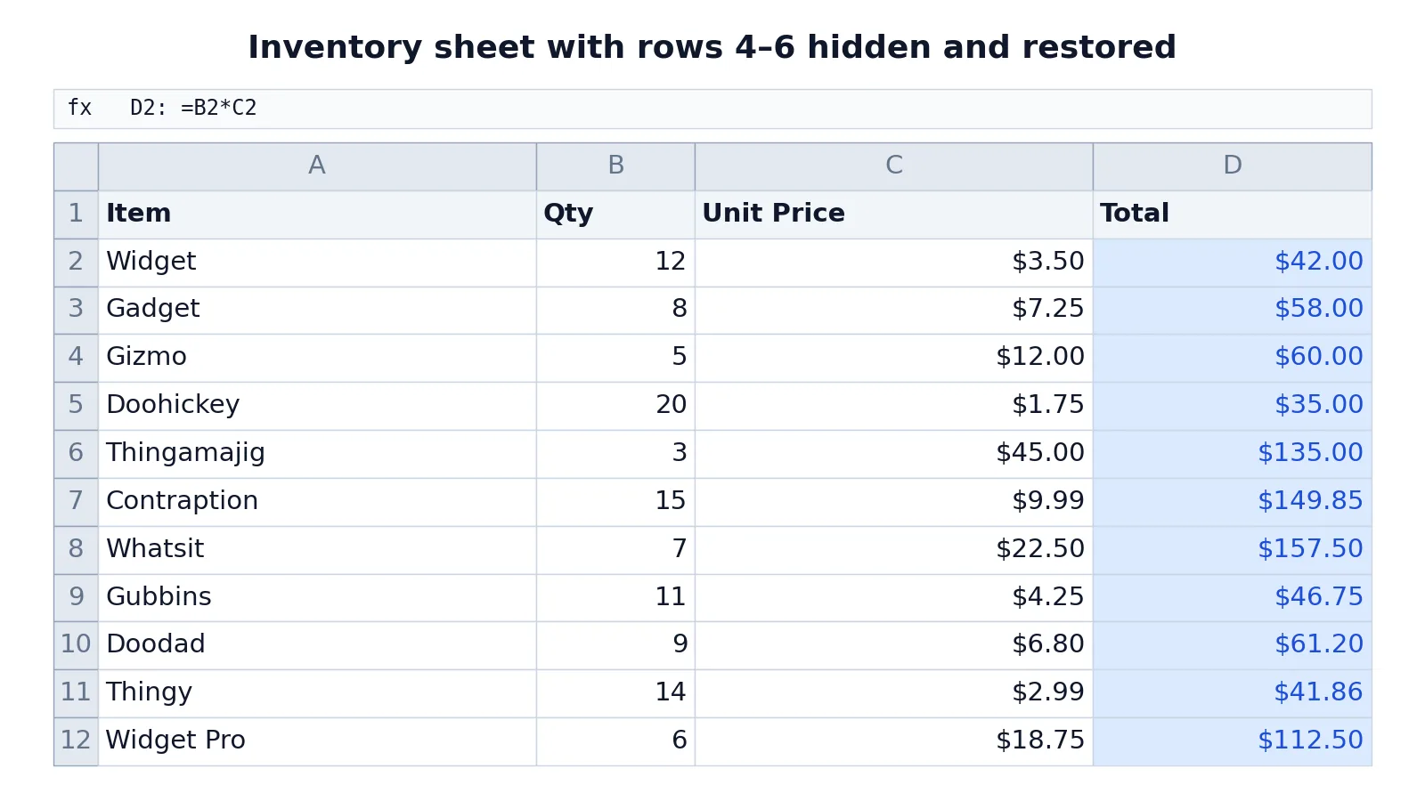
The table below is a 12-row inventory sheet with an Item column, a Qty column, a Unit Price column, and a Total column. Each Total cell multiplies quantity by unit price.

Row	A	B	C	D
1	Item	Qty	Unit Price	Total
2	Widget	12	3.5	`=B2*C2` -> displays $42.00
3	Gadget	8	7.25	`=B3*C3` -> displays $58.00
4	Gizmo	5	12	`=B4*C4` -> displays $60.00
5	Doohickey	20	1.75	`=B5*C5` -> displays $35.00
6	Thingamajig	3	45	`=B6*C6` -> displays $135.00
7	Contraption	15	9.99	`=B7*C7` -> displays $149.85
8	Whatsit	7	22.5	`=B8*C8` -> displays $157.50
9	Gubbins	11	4.25	`=B9*C9` -> displays $46.75
10	Doodad	9	6.8	`=B10*C10` -> displays $61.20
11	Thingy	14	2.99	`=B11*C11` -> displays $41.86
12	Widget Pro	6	18.75	`=B12*C12` -> displays $112.50

The formula in every Total cell follows the same pattern:

$$D_n = B_n \times C_n$$

Suppose rows 4, 5, and 6 are hidden. The row headers jump from 3 to 7, and a double line sits between them. The visible sheet shows Widget at $42.00, Gadget at $58.00, then Contraption at $149.85. The Gizmo, Doohickey, and Thingamajig totals of $60.00, $35.00, and $135.00 are still in the file, just not displayed.

After Select All > Format > Hide & Unhide > Unhide Rows, all 12 rows are visible again and the totals read $42.00, $58.00, $60.00, $35.00, $135.00, $149.85, $157.50, $46.75, $61.20, $41.86, and $112.50 in order. The same result can be reproduced outside Excel by reindexing a DataFrame to restore the missing rows, which is a useful check when you are auditing a sheet you did not build.

Other Ways to Do It

The Select All and Format menu method is the most reliable because it does not depend on guessing where the hidden rows are. A few alternatives exist.

Right-click on selected headers. Select the row headers surrounding the hidden rows, right-click, and choose Unhide [1]. This is the quickest option when you know exactly which rows are missing.

Double-click the double line. Double-click the double line between the two rows where hidden rows exist [1]. This works well for a single hidden row or a small block.

Go To Special for hidden cells. If you need to find cells that live inside hidden rows or columns, use Find & Select > Go To Special on the Home tab, choose Visible cells only, and click OK [3]. This selects the visible cells and marks the borders of rows and columns adjacent to hidden ones with a white border, which helps you locate the gap [3]. Note that this feature is not available in Excel for the web [3].

Unhide the first row. If row 1 itself is hidden, Select All still works, and so does selecting row 2 and dragging upward before right-clicking. Microsoft documents unhiding the first row or column as a separate case because there is no header above it to select [1].

If your sheet has blank rows mixed in with hidden ones and you want them gone for good, see how to delete blank rows in Excel. If you want to keep certain rows visible while scrolling instead of hiding others, how to freeze rows and columns in Excel is the better tool.

Troubleshooting

Unhide Rows is grayed out. The worksheet is probably protected. Unprotect the sheet first, then repeat the steps. If you cannot unprotect it, you need the password from whoever set it.

Rows come back but the data looks wrong. Check for filters. A filter hides rows without changing the row headers, so the double line indicator is absent. Clear the filter instead of unhiding. The guide on how to filter in Excel explains how filters interact with row visibility.

Only some rows return. You may have selected a partial range instead of the whole sheet. Click Select All and repeat the Format > Hide & Unhide > Unhide Rows sequence.

The row numbers still skip. Grouped rows behave differently from hidden rows. Look for outline brackets or a plus sign in the left margin and expand the group instead.

Nothing happens at all. Confirm you are on the correct sheet. Hidden rows on another worksheet are unaffected by what you do on the active one.

Common Mistakes

Selecting only the visible rows above the gap. The selection must include the headers on both sides of the hidden rows. Fix: drag across the header above and the header below before right-clicking.
Confusing hidden rows with filtered rows. Filters hide rows without leaving a double line, so Unhide does nothing. Fix: clear the filter from the Data tab.
Assuming hidden rows are deleted. The data is still present and still feeds formulas. Fix: unhide instead of retyping the data.
Printing before unhiding. In Excel for the web, hidden rows and columns are excluded from the printout [2]. Fix: unhide first, then print.
Forgetting row 1. There is no header above row 1 to select. Fix: use Select All, or select row 2 and drag upward.
Ignoring sheet protection. A protected sheet blocks the Unhide command. Fix: unprotect the sheet, unhide, then re-protect it if needed.

Limitations

Unhiding restores visibility, not content. If a row was deleted, no unhide command will bring it back, and the row numbers will not show a gap, because Excel renumbers the rows below it. Unhiding also does not change any values, so if a total looked wrong while the row was hidden, it will look exactly the same once revealed.

The Go To Special approach for locating hidden cells is not available in Excel for the web [3], so browser users are limited to the header selection and Format menu methods. Row visibility is also stored per worksheet, which means unhiding rows on one sheet has no effect on any other sheet in the workbook.

Frequently Asked Questions

How do I unhide Excel rows when the row numbers skip?

Click the Select All button at the top-left corner of the sheet, then go to Home > Format > Hide & Unhide > Unhide Rows. This reveals every hidden row on the active worksheet at once. If the numbers still skip afterward, a filter or row group is controlling visibility. Deleted rows never leave a gap, because Excel renumbers the rows below them.

How do you unhide rows in Excel for just one hidden row?

Select the row headers directly above and below the hidden row, right-click the selection, and choose Unhide [1]. You can also double-click the double line between the two visible rows [1]. Both methods work on a single row and on a contiguous block.

Why is Unhide Rows grayed out?

The worksheet is most likely protected. Protection disables structural changes, including hiding and unhiding rows. Unprotect the sheet from the Review tab, repeat the unhide steps, then apply protection again if you need it.

How do I unhide cells in Excel that are inside hidden rows?

You cannot unhide individual cells. Cells become invisible only because their entire row or column is hidden, so you unhide the row or column and the cells reappear. To locate cells that sit in hidden rows, use Home > Find & Select > Go To Special > Visible cells only [3].

Does unhiding rows change my formulas or data?

No. Hiding and unhiding only affect display. Every value, formula, and reference stays intact while a row is hidden, which is why totals in other cells do not change when you reveal the row. If you need to remove rows permanently, use how to remove duplicates in Excel or delete the rows outright.