Negative Binomial Distribution: Formula and Examples

By Dr. Zubair Khalid, DVM, MS, PhD · 2026-10-03

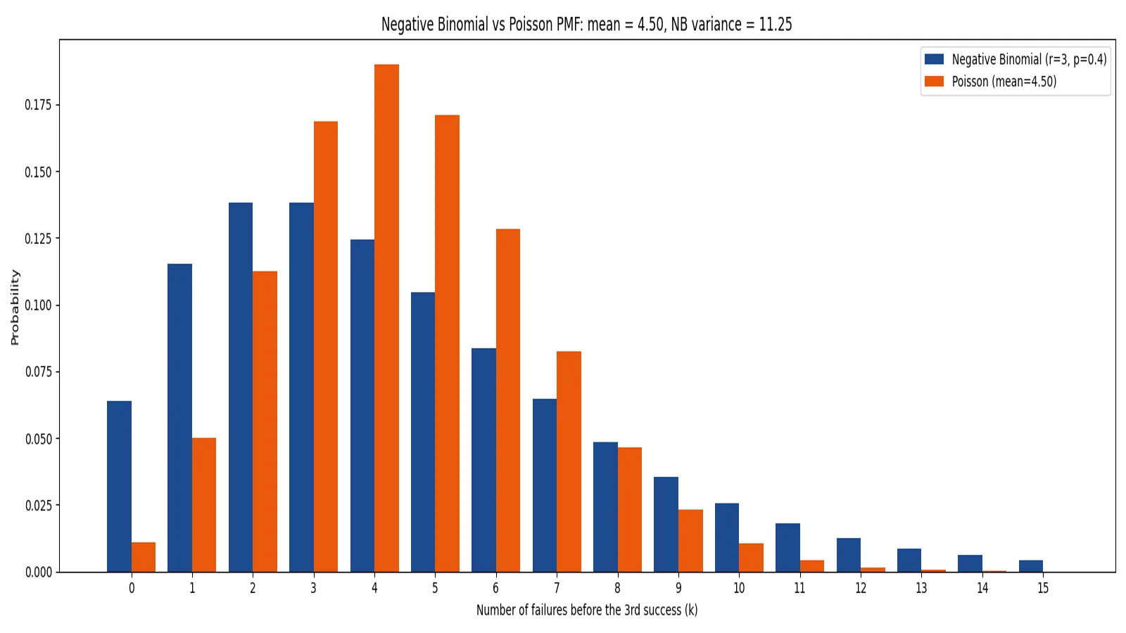
The negative binomial distribution models the number of failures that occur before a fixed number of successes is reached in a sequence of independent trials. It is the standard choice when you count events and the variance of your data is larger than its mean, a condition called overdispersion. This article covers the formula, a fully worked example, and how the negative binomial differs from the Poisson.

Quick Answer

The negative binomial distribution counts failures before the $r$-th success, where each trial succeeds with probability $p$ [1].
Its probability mass function is $P(X=k) = \binom{k+r-1}{k} p^r (1-p)^k$ for $k = 0, 1, 2, \dots$
The mean is $r(1-p)/p$ and the variance is $r(1-p)/p^2$, so the variance is always larger than the mean.
Use it for overdispersed counts, where the Poisson assumption that variance equals the mean fails.
In Excel, NEGBINOM.DIST(k, r, p, FALSE) returns the probability of exactly $k$ failures.

What the Negative Binomial Distribution Means

In plain terms, imagine repeating a trial that either succeeds or fails. You keep going until you have collected a target number of successes. The negative binomial distribution tells you how many failures you will rack up along the way.

The precise statistical definition is this. The negative binomial random variable with parameters $n$ and $p \in (0,1)$ is the number of extra independent trials beyond $n$ required to accumulate a total of $n$ successes, where the probability of success on each trial is $p$ [1]. Equivalently, it is the number of failures encountered while accumulating $n$ successes during independent trials of an experiment that succeeds with probability $p$ [1]. Many textbooks and software packages write the success target as $r$ instead of $n$. This article uses $r$ to avoid confusion with the binomial distribution's trial count.

The name comes from the binomial coefficient $\binom{k+r-1}{k}$ that appears in the formula. It is a binomial-style coefficient, and the "negative" refers to the negative exponent in the generating function, not to anything negative about the data.

How It Works

The probability mass function gives the probability of observing exactly $k$ failures before the $r$-th success:

$$P(X=k) = \binom{k+r-1}{k} p^r (1-p)^k, \quad k = 0, 1, 2, \dots$$

Each symbol has a specific job:

Symbol	Meaning
$k$	Number of failures observed before the $r$-th success
$r$	Target number of successes you stop at
$p$	Probability of success on a single trial
$1-p$	Probability of failure on a single trial
$\binom{k+r-1}{k}$	Number of orderings of $k$ failures and $r-1$ successes before the final success

The factor $p^r$ accounts for the $r$ successes. The factor $(1-p)^k$ accounts for the $k$ failures. The binomial coefficient counts how many ways those failures and successes can be arranged before the last trial, which must be a success.

The mean and variance follow directly:

$$\text{Mean} = \frac{r(1-p)}{p}, \qquad \text{Variance} = \frac{r(1-p)}{p^2}$$

Because $p$ is between 0 and 1, the variance is always greater than the mean. That single property is why the negative binomial is the go-to model for overdispersed counts. If you want the mirror-image setup, where you fix the number of trials instead of the number of successes, see the binomial distribution formula and examples.

Worked Example

Suppose 12 clinics each run a screening process until they record 3 successes, with a per-attempt success probability of $p = 0.4$. The table records how many failures each clinic logged before its 3rd success.

Clinic	Failures before 3rd success
C01	4
C02	2
C03	7
C04	3
C05	5
C06	1
C07	6
C08	2
C09	4
C10	8
C11	3
C12	5

Take clinic C01, which recorded $k = 4$ failures. With $r = 3$ and $p = 0.4$, the PMF is:

$$P(X=4) = \binom{4+3-1}{4} \cdot 0.4^3 \cdot (1-0.4)^4$$

The binomial coefficient is $\binom{6}{4} = 15$. Substituting:

$$15 \cdot 0.4^3 \cdot 0.6^4 = 0.1244$$

So the probability that a clinic logs exactly 4 failures before its 3rd success is 0.1244.

The theoretical mean is $r(1-p)/p = 3 \cdot 0.6 / 0.4 = 4.5000$. The theoretical variance is $r(1-p)/p^2 = 3 \cdot 0.6 / 0.16 = 11.2500$.

Now compare with the observed data. The mean of the 12 clinic counts is 4.1667 and the sample variance is 4.5152. Under a Poisson model, the variance would be forced to equal the mean, so $Var_{Poisson} = 4.1667$. The variance ratio is $4.5152 / 4.1667 = 1.0836$, which is above 1 and signals mild overdispersion.

Here is the calculation in Python, with the equivalent calls in Excel and R:

import math
r, p, k = 3, 0.4, 4
pmf = math.comb(k + r - 1, k) * p**r * (1 - p)**k
print(round(pmf, 4))

Output:

0.1244

The Excel function NEGBINOM.DIST returns the same 0.1244, which confirms the hand calculation.

How to Interpret It

The PMF value 0.1244 is a probability for one specific outcome, not a summary of the whole distribution. To judge whether a count is unusual, compare it with the mean of 4.5. A clinic with 8 failures sits well above the mean, and the negative binomial's heavier right tail makes that outcome more plausible than a Poisson model would suggest.

The variance ratio is the practical diagnostic. When the sample variance divided by the sample mean is close to 1, the Poisson fits. When it is clearly above 1, as in this example, the negative binomial is the better description. The distribution is right skewed, so a small number of units will show large counts. That shape is common in count data and is covered in right skewed distribution meaning and examples.

When to Use It (and when not to)

Use the negative binomial when you are counting events and the variance exceeds the mean. Typical cases include counts of defects per batch, insurance claims per policyholder, RNA sequencing reads per gene, and hospital admissions per region.

Use it when the process can be framed as waiting for a fixed number of successes, or when you need a count model that allows extra variability beyond the Poisson. The Poisson distribution formula and examples covers the equal mean and variance case.

Do not use it when the variance equals the mean, since the Poisson is simpler and sufficient. Do not use it when the number of trials is fixed in advance, because that is the binomial setup. Do not use it when events are strongly dependent on each other, since the model assumes independent trials. If you need the special case where you stop at the first success, see the geometric distribution formula and examples.

Negative Binomial vs Poisson

The two distributions both model counts, but they differ in one decisive way: the relationship between mean and variance.

Feature	Negative Binomial	Poisson
Parameterization	$r$ successes, probability $p$	Rate $\lambda$
Mean	$r(1-p)/p$	$\lambda$
Variance	$r(1-p)/p^2$	$\lambda$
Variance vs mean	Variance always greater than mean	Variance equals mean
Handles overdispersion	Yes	No
Typical use	Overdispersed counts	Equally dispersed counts

The Poisson PMF is $p(x;\lambda) = e^{-\lambda}\lambda^x / x!$ [2]. Its single parameter $\lambda$ sets both the mean and the variance, so it cannot absorb extra spread. The negative binomial adds a second parameter, which lets the variance float free of the mean. That flexibility is why it dominates in fields like genomics, where counts are routinely overdispersed. For a deeper look at that application, see negative binomial models in RNA-seq.

Common Mistakes

Confusing the negative binomial with the binomial. The binomial fixes the number of trials and counts successes [3]. The negative binomial fixes the number of successes and counts failures. Fix: check which quantity is held constant before choosing a formula.
Mixing up $k$ and $r$. Some software uses n for the success target and others use size. Fix: read the function signature and confirm which argument is the success count.
Forgetting that $k$ starts at 0. The first outcome is zero failures before the $r$-th success. Fix: include $k = 0$ when you sum probabilities.
Assuming the variance equals the mean. That is the Poisson property, not the negative binomial property. Fix: compute $r(1-p)/p^2$ and compare it with the mean.
Using the wrong success probability. If you enter $1-p$ where $p$ belongs, the answer will be wrong. Fix: confirm that $p$ is the probability of the event you are counting as a success.
Treating a single PMF value as a p-value. The PMF gives the probability of one exact count. Fix: sum the PMF over the range you care about to get a cumulative probability.

Limitations

The negative binomial assumes independent trials with a constant success probability. Real count data often violates both. If the probability drifts over time, or if events cluster, the model will understate or overstate the tail. It also assumes the variance grows as a specific quadratic function of the mean, which may not match every dataset.

The distribution is defined only for non-negative integers, so it cannot describe continuous measurements. When overdispersion is severe, a single negative binomial may still be too light-tailed, and you may need a mixture or a zero-inflated variant. Always check the fit against your observed counts before relying on the model for inference.

Frequently Asked Questions

What is the difference between the negative binomial and the Poisson distribution?

The Poisson forces the variance to equal the mean. The negative binomial allows the variance to exceed the mean, which makes it suitable for overdispersed counts. If your data show a variance-to-mean ratio well above 1, the negative binomial usually fits better.

What do the parameters r and p mean?

$r$ is the target number of successes at which you stop counting, and $p$ is the probability of success on each individual trial. Together they set the mean $r(1-p)/p$ and the variance $r(1-p)/p^2$.

How do I calculate the negative binomial distribution in Excel?

Use NEGBINOM.DIST(k, r, p, FALSE) for the probability of exactly $k$ failures, or TRUE for the cumulative probability. For $k = 4$, $r = 3$, and $p = 0.4$, the function returns 0.1244. You can also check related discrete probabilities with the binomial distribution calculator.

When should I use the negative binomial instead of the Poisson?

Use the negative binomial when the sample variance is clearly larger than the sample mean. A variance ratio near 1 supports the Poisson. A ratio noticeably above 1, such as 1.0836 in the clinic example, points toward the negative binomial.

Can the negative binomial model zero counts?

Yes. The value $k = 0$ is a valid outcome and represents reaching the target number of successes with no failures at all. Its probability is $p^r$, which is the chance that the first $r$ trials are all successes.