Bernoulli Distribution: Definition, Formula and Examples

By Dr. Zubair Khalid, DVM, MS, PhD · 2026-10-03

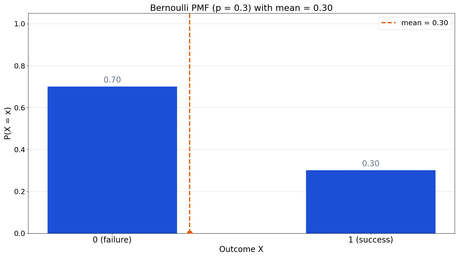
The Bernoulli distribution is the probability distribution of a single trial that has exactly two possible outcomes, usually labeled success (1) and failure (0). It is described by one parameter, $p$, the probability of success. Every binary event you can think of, from a coin flip to whether a visitor clicks an ad, can be modeled this way.

Quick Answer

A Bernoulli random variable takes only two values: 1 (success) and 0 (failure) [1].
It has one parameter, $p$, the probability of a single success, while $1-p$ is the probability of a single failure [2].
The probability mass function is $P(X=1)=p$ and $P(X=0)=1-p$ [2][3].
The mean is $E[X]=p$ and the variance is $\text{Var}(X)=p(1-p)$ [4].
A binomial distribution with $n=1$ trial is exactly a Bernoulli distribution [1][3].

What the Bernoulli Distribution Means

In plain terms, the Bernoulli distribution answers one question: what is the chance of a single yes-or-no outcome? You run the trial once. You record whether the event happened. That is the whole distribution.

The precise statistical definition: a discrete random variable $X$ follows a Bernoulli distribution with parameter $p$ if its support is $\{0, 1\}$ and its probability mass function assigns $1-p$ to $k=0$ and $p$ to $k=1$, for $0 \le p \le 1$ [2]. You write this as $X \sim \text{Bernoulli}(p)$.

The two outcomes are conventionally called success and failure, but the labels are arbitrary. A "success" can be a defective part, a missed free throw or a fraudulent transaction. What matters is that you pick one outcome to code as 1 and keep that coding consistent.

This distribution is the simplest building block for other discrete distributions. Sequences of independent Bernoulli trials generate the binomial, geometric and negative binomial distributions [3]. If you want the wider picture, see Probability Distributions: Definition, Types and Examples.

How It Works

The Bernoulli probability mass function (PMF) gives the probability of each possible outcome:

$$ P(X = k) = \begin{cases} 1 - p & \text{if } k = 0 \\ p & \text{if } k = 1 \end{cases} $$

Each symbol means the following:

$X$ is the random variable, the outcome of the single trial.
$k$ is the value you are asking about, either 0 or 1.
$p$ is the probability of success, a number between 0 and 1.
$1-p$ is the probability of failure, often written as $q$.

A compact way to write the same function for $k \in \{0,1\}$ is $P(X=k) = p^{k}(1-p)^{1-k}$. When $k=1$ the second factor becomes 1, leaving $p$. When $k=0$ the first factor becomes 1, leaving $1-p$.

The mean and variance follow directly from the two-point support [4]:

$$E[X] = p \qquad \text{Var}(X) = p(1-p)$$

The mean equals the success probability because the only nonzero value is 1, weighted by $p$. The variance is largest when $p = 0.5$ and shrinks toward zero as $p$ approaches 0 or 1, because the outcome becomes more predictable.

Worked Example

Suppose you track 10 click-through trials for a banner ad, where 1 means the visitor clicked and 0 means they did not. The observed sequence is below.

Trial	1	2	3	4	5	6	7	8	9	10
Click	1	0	1	0	0	1	0	0	1	0

You model each trial as a Bernoulli random variable with $p = 0.3$. Here is the full walkthrough.

Trial setup: $n = 10$ trials, 4 successes, $p = 0.3$.
PMF at $X=1$: $P(X=1) = p = 0.3$, which is 0.3000.
PMF at $X=0$: $P(X=0) = 1 - p = 1 - 0.3 = 0.7000$.
Mean: $E[X] = p = 0.3$, which is 0.3000.
Variance: $\text{Var}(X) = p(1-p) = 0.3 \times 0.7 = 0.2100$.
Standard deviation: $\text{SD} = \sqrt{0.2100} = 0.4583$.
Sample proportion: $\hat{p} = 4/10 = 0.4000$.

The sample proportion of 0.4000 is your estimate from the data. The parameter $p = 0.3$ is the assumed true probability. They differ because 10 trials is a small sample, and sampling variability is expected.

You can reproduce these numbers in Python with SciPy [2]:

from scipy.stats import bernoulli
rv = bernoulli(p=0.3)
print(f"P(X=1)={rv.pmf(1):.4f}, P(X=0)={rv.pmf(0):.4f}, mean={rv.mean():.4f}, variance={rv.var():.4f}")

Output:

P(X=1)=0.3000, P(X=0)=0.7000, mean=0.3000, variance=0.2100

In Excel, the same values round to 0.3 for $P(X=1)$, 0.7 for $P(X=0)$, 0.3 for the mean and 0.21 for the variance.

How to Interpret It

The PMF tells you the long-run relative frequency of each outcome if you repeated the single trial many times under identical conditions. With $p = 0.3$, roughly 30 percent of trials should be successes across a large number of repetitions.

The mean of 0.3 is not a value the variable can take. It is the expected value, the average of 0s and 1s over many trials. The variance of 0.21 measures how spread out those 0s and 1s are around that average.

The parameter $p$ is a property of the process, not of your sample. Your data gives you $\hat{p}$, an estimate. As the number of trials grows, $\hat{p}$ tends to get closer to $p$. This distinction between parameter and estimate is central to Fundamental Statistics: Core Concepts Explained.

When to Use It (and when not to)

Use the Bernoulli distribution when all of these hold:

There is exactly one trial or one observation.
The outcome is binary, coded as 0 or 1.
The probability of success $p$ is fixed for that trial.
You care about the outcome of that single trial, not a count across many.

Do not use it when you have more than one trial and want the total number of successes. That situation calls for the binomial distribution, which is the sum of $n$ independent Bernoulli random variables [1]. If you are counting trials until the first success, use the geometric distribution. If you are counting trials until the $r$-th success, use the negative binomial.

The Bernoulli distribution also assumes the outcome is genuinely binary. If your variable has three or more categories, or is continuous, it does not apply.

Bernoulli Distribution vs Binomial Distribution

The binomial distribution is the natural comparison because the two are directly related. A binomial distribution with $n = 1$ is a Bernoulli distribution [1][3].

Feature	Bernoulli	Binomial
Number of trials	1	$n$ trials
Random variable	Outcome of one trial (0 or 1)	Number of successes in $n$ trials
Parameters	$p$	$n$ and $p$
Possible values	0, 1	0, 1, ..., $n$
Mean	$p$	$np$
Variance	$p(1-p)$	$np(1-p)$

If you need counts across many trials, the Binomial Distribution: Formula, Mean and Examples article covers the full formula. You can also run numbers quickly with the Binomial Distribution Calculator.

Common Mistakes

Confusing the parameter with the sample proportion. The parameter $p$ is the true probability, while $\hat{p}$ is what you measured. Fix: report both and label them clearly.
Using Bernoulli when you have multiple trials. If you sum outcomes across trials, you need a binomial model. Fix: check whether your variable counts successes or records a single outcome.
Assuming the mean must be an observable value. The mean of 0.3 is not a possible outcome. Fix: interpret the mean as a long-run average, not a single result.
Forgetting that $p$ must stay between 0 and 1. A probability outside that range is invalid [2]. Fix: validate your parameter before computing anything.
Treating dependent trials as independent. Bernoulli trials assume a fixed $p$ per trial. Fix: if the probability changes between trials, the simple model does not hold.
Ignoring small-sample noise. With 10 trials, $\hat{p}$ can differ a lot from $p$. Fix: use larger samples before drawing firm conclusions.

Limitations

The Bernoulli distribution describes only a single binary trial. It cannot represent counts, multi-category outcomes or continuous measurements. If your question involves more than one trial, you need a distribution built from repeated Bernoulli trials, such as the binomial or geometric.

It also assumes a fixed success probability and independence across any repeated trials. Real processes often violate this. Click rates shift with time of day, defect rates change with machine wear, and outcomes can be correlated within groups. When those conditions fail, a Bernoulli or binomial model can understate or overstate variability, so treat the results as an approximation and check your assumptions.

Frequently Asked Questions

What is the difference between a Bernoulli distribution and a Bernoulli random variable?

A Bernoulli random variable is the variable itself, the thing that takes the value 0 or 1. The Bernoulli distribution is the set of probabilities attached to those values. You say $X$ is a Bernoulli random variable and $X$ follows a Bernoulli distribution with parameter $p$ [1].

What is the Bernoulli distribution formula?

The PMF is $P(X=1)=p$ and $P(X=0)=1-p$ [2][3]. The mean is $p$ and the variance is $p(1-p)$ [4]. These three facts cover almost every calculation you will do with a single binary trial.

Is the Bernoulli distribution the same as the binomial distribution?

No, but they are closely linked. A binomial distribution with $n=1$ trial is a Bernoulli distribution [1]. The binomial generalizes the Bernoulli to any number of independent trials and counts the total successes.

Can the Bernoulli distribution have a mean other than 0 or 1?

Yes. The mean is $p$, which can be any value between 0 and 1, such as 0.3. The mean is an expected value, so it does not need to be one of the two possible outcomes.

What is the variance of a Bernoulli distribution?

The variance is $p(1-p)$ [4]. It reaches its maximum of 0.25 when $p = 0.5$ and approaches 0 as $p$ gets close to 0 or 1. For $p = 0.3$, the variance is 0.21 and the standard deviation is about 0.4583.

References

Bernoulli & Binomial Random Variables - Data Science Discovery
scipy.stats.bernoulli, SciPy v1.18.0 Manual
Bernoulli Distribution
6.5: Bernoulli Distribution - Statistics LibreTexts/06%3A_Discrete_Random_Variables/6.05%3A_Bernoulli_Distribution)