What is Dr. Zubair Khalid's research focus?

Dr. Zubair Khalid specializes in molecular virology, mRNA vaccine development, and computational biology, with a focus on avian pathogens like IBDV and Avian Reovirus.

Where is Dr. Zubair Khalid currently working?

Dr. Zubair Khalid is a Postdoctoral Research Associate at the University of Maryland (UMD), specifically within the Department of Animal and Avian Sciences.

Right Skewed Distribution: Meaning and Examples

By Dr. Zubair Khalid, DVM, MS, PhD · 2026-09-20

A right skewed distribution is a frequency distribution with a long tail extending toward higher values, in which most observations cluster at the low end of the scale and a small number of large values stretch the curve to the right. In a right-skewed dataset the mean is greater than the median, and the mode is the lowest of the three measures of center.

That single sentence carries a lot of practical weight. Skewness decides whether you report a mean or a median, whether a t-test is defensible, whether a log transformation will help or hurt, and whether a reviewer will accept your statistics. Biological measurements are skewed far more often than they are symmetric, and the skew usually runs to the right. Colony counts, enzyme rates, viral loads, body burdens of contaminants, and daily blood product usage all pile up near zero and trail off toward large values [1][2]. Recognizing the shape early saves you from reporting a mean that no individual in your study actually resembles.

What Skewness Means

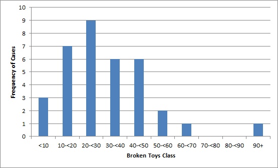
Histogram with a long tail extending to the right, labeled as right-skewed — A right-skewed histogram has its peak on the left and a long tail stretching toward higher values on the right. Image: Monika Wahi, CC BY-SA 4.0, via Wikimedia Commons.

Skewness is a measure of asymmetry in a distribution. A perfectly symmetric distribution, such as the classic Gaussian bell curve, has a skewness of zero. When the bulk of the data sits on the left and the tail stretches right, the distribution is right skewed. When the bulk sits on the right and the tail stretches left, it is left skewed, also written as left skewness.

The direction of skew is named for the tail, not for where the peak sits. This is the single most common point of confusion. A right-skewed histogram has its tallest bars on the left side of the x-axis and its thin, sparse tail on the right. A left-skewed histogram has its tallest bars on the right and its thin tail on the left.

The Mean, Median, and Mode Ordering

In a right-skewed distribution, the three measures of center line up in a predictable order:

Mode is lowest. It marks the peak, where the most common values sit.
Median is in the middle. It splits the data in half by count, so extreme values cannot drag it far.
Mean is highest. It sums every value, so a few very large observations pull it upward.

In a left-skewed distribution the order reverses. The mean falls below the median, which falls below the mode. The gap between mean and median is a quick, useful diagnostic. If someone hands you a summary table showing a mean of 42 and a median of 18, you can be confident the underlying data are right skewed without ever seeing a histogram.

Why the Mean Moves and the Median Does Not

The mean is an arithmetic average. Every observation contributes its full value divided by the sample size. A single colony count of 4,000 in a dataset of 50 plates adds 80 to the mean all by itself. The median only cares about rank order. That same 4,000 could be 400 or 40,000 and the median would not budge, as long as it remains the largest value.

This is why the median is called robust. Robustness means insensitivity to extreme values. When a distribution is heavily skewed, the median describes the typical case far better than the mean does. Reporting only the mean of a right-skewed variable gives a number that may exceed most of the observations in the dataset.

Right Skew Versus Left Skew: A Comparison

The table below summarizes the two mirror-image shapes and the practical choices that follow from each.

Feature	Right skew (positive skew)	Left skew (negative skew)
Tail direction	Long tail toward higher values	Long tail toward lower values
Peak location	Left side of the axis	Right side of the axis
Mode	Lowest of the three	Highest of the three
Median	Middle	Middle
Mean	Highest of the three	Lowest of the three
Mean versus median	Mean greater than median	Mean less than median
Typical biological example	Colony counts, enzyme activity, viral load, body burden	Age at death in a cohort, ceiling-limited scores, some latency measures
Common transformation	Log or Box-Cox	Square, cube, or reflect-then-log
Typical test choice	Median or rank-based tests, or parametric tests after a justified transformation	Same logic, mirrored

The two shapes are not equally common in biology. Positive skew dominates because many biological quantities have a natural floor at zero and no matching ceiling. A count cannot be negative. An enzyme rate cannot be negative. A viral load cannot be negative. Values can, however, be arbitrarily large. That one-sided constraint produces the long right tail again and again.

Why Biology Produces Right Skew So Often

Several distinct mechanisms generate right-skewed data, and knowing which one applies to your variable helps you choose the right analysis.

Multiplicative Processes

When a quantity grows by repeated multiplication rather than repeated addition, its distribution tends toward the log-normal. A log-normal distribution is one whose logarithm is normally distributed, and it is always right skewed. Bacterial growth over time, the accumulation of a metabolite through several enzymatic steps, and the product of many small independent random effects all behave this way. Because the underlying process is multiplicative, the natural scale for analysis is logarithmic.

Floor Effects and Count Data

Any variable bounded below at zero with no upper bound will tend to skew right. Microbiome abundance counts are a textbook case. Sequencing reads per taxon pile up at low values and a handful of dominant taxa absorb a large share of the reads, producing a distribution that is skewed to the right and overdispersed [1]. Overdispersion means the variance exceeds the mean, which violates the assumptions of simple Poisson models and requires either robust standard errors or a different model family.

Rare Large Events

Some biological variables are shaped by infrequent, high-magnitude events. Daily red blood cell usage in a hospital is one. Most days require a modest number of units, but occasional days involve a massively transfused patient, and those days push the distribution far to the right. A study of 241,957 units transfused over 2,557 days found that log-normal and gamma distributions described daily usage better than the normal distribution, and that the highest-usage days were significantly more likely to include at least one ultramassively transfused patient [2]. Inventory planning based on a normal assumption would systematically underestimate demand on those days.

Ecological and Evolutionary Patterns

Right skew appears at the scale of whole ecosystems. A global analysis of forest plots across five continents found that in warmer and wetter forests, aboveground biomass and woody productivity were more right skewed, with a long tail toward large trees [3]. Most trees are small, and a few giants hold a disproportionate share of the biomass. The same pattern appears in thermal sensitivity across microbial species, where the distribution of activation energy values is typically right skewed [4].

Reading a Histogram

A histogram plots value ranges on the horizontal axis and frequency on the vertical axis. To identify skew by eye, follow three steps.

Find the tallest bar. Note which side of the axis it sits on.
Follow the curve outward in both directions. One side will drop off steeply, the other will taper gradually.
The tapering side is the tail. If the tail points right, the distribution is skewed right.

A quick sanity check uses the mean and median. If the reported mean exceeds the reported median, the data are almost certainly right skewed. If the mean is below the median, suspect left skew.

One caution about visual inspection. Small samples produce lumpy histograms, and a single outlier can create the appearance of a tail that would not persist with more data. Skewness is a property of the population, and sample skewness is an estimate. With fewer than roughly 30 observations, treat visual impressions as suggestive rather than conclusive.

Testing and Quantifying Skewness

Formal assessment usually combines a numeric skewness statistic with a normality test.

The skewness statistic standardizes the third moment of the distribution. A value near zero indicates symmetry. Positive values indicate right skew and negative values indicate left skew. There is no universal cutoff, but many practitioners treat absolute values above roughly 1 as substantial and above roughly 2 as severe. These thresholds are conventions, not laws, and they depend on sample size.

Normality tests such as the Shapiro-Wilk test ask whether the data are consistent with a Gaussian distribution. A significant result means the normality assumption is questionable. These tests are sensitive to sample size in both directions. Very large samples flag trivial deviations, and very small samples lack the power to detect real ones. This is why formal tests should accompany a histogram and a mean-versus-median comparison rather than replace them.

Skewness also interacts with kurtosis, which measures tail heaviness. One methodological study of neuroendocrine data noted that the hardest distributions to normalize were those with a high ratio of kurtosis to skewness [5]. In other words, a heavy-tailed right-skewed variable is more stubborn than a mildly skewed one.

Transformations: What Works and What Does Not

Because many parametric tests assume normally distributed residuals, researchers often transform skewed variables before analysis. The goal is to compress the long tail and pull the distribution toward symmetry.

The Log Transformation

The logarithmic transformation is the default for right-skewed data. Taking the log of each value compresses large values far more than small ones, which shortens the right tail. For a log-normal variable, the log transformation produces an exactly normal distribution, which is why the log-normal is such a convenient model.

A study of external quality assessment data across five analytes used a formula based on log transformation under the assumption that the analytes had skewed distributions, and estimated inter-laboratory reference change values ranging from 13.3% to 203% on the positive side [6]. That is a concrete illustration of how assuming a skewed, log-normal shape changes the numbers you report.

When Log Transformation Fails

Log transformation is not a universal fix, and the literature has grown increasingly skeptical of reflexive use.

One analysis of proficiency testing data challenged the common practice of log-transforming GMO test results. Across 56 datasets containing 3,178 reported results, 41 datasets were already normally distributed on the raw scale, and 10 more could not be shown to deviate significantly from normality on either scale. Only five datasets became normal after log transformation, and those turned out to be multimodal because of technical problems with the methods used [7]. The practical lesson is that log transformation is often unnecessary and should be applied cautiously.

A separate methodological review went further, arguing that the common belief that log transformation reduces variability and restores normality is usually not true, and that standard tests run on log-transformed data often answer a question that is not relevant to the original scale [8]. The authors recommended distribution-free approaches such as generalized estimating equations in many situations.

Box-Cox and Adaptive Methods

The Box-Cox transformation is a family of power transformations that includes the log, square root, and inverse as special cases. Rather than guessing which power to use, the analyst estimates it from the data. Applied to positively skewed neuroendocrine data, Box-Cox transformation brought roughly two-thirds of cases into strict alignment with a Gaussian distribution, and the remainder improved substantially even when they did not fully normalize [5].

Newer approaches tune the transformation per feature rather than per dataset. Metabolomic data illustrate why this matters. A large-scale study found that metabolic features have diverse distribution types, and that most of them cannot be normalized correctly with conventional log or square root transformations. The authors proposed an adaptive Box-Cox transformation that tunes a power parameter based on a normality test result, and it outperformed conventional approaches for both positively and negatively skewed data [9].

Transformation choices can also change biological conclusions, not just statistical ones. In a study of litter size in Landrace pigs, Box-Cox transformation shifted the skewness statistic from -0.46 to -0.02 and changed heritability estimates for total number born from 0.118 to 0.125, with larger relative changes in variance-based traits [10]. Transformation is a modeling decision with consequences.

Geometric Means and Log-Normal Data

When data are log-normal, the appropriate summary of central tendency is the geometric mean. The geometric mean is the nth root of the product of n values, and it equals the exponential of the mean of the logged values. It is always less than or equal to the arithmetic mean, with the gap widening as skew increases.

Geometric means are standard for titers, viral loads, and dilution series. Meta-analytic methods have been developed specifically to combine studies that report results on the raw scale with studies that report them on the log scale, and to produce a meta-analysis of ratios of geometric means when every study reports skewed data on the raw scale. The authors concluded that an approach based on a log-normal assumption for the raw data is reasonably robust across different true distributions [11].

The practical rule is straightforward. If you log transform for analysis, report the geometric mean and a multiplicative measure of spread rather than back-transforming a standard deviation, which produces a nonsensical interval.

Choosing a Statistical Test

The choice of test follows from the shape of the data and the question being asked.

For two-group comparisons of right-skewed data, the Wilcoxon-Mann-Whitney test is a common rank-based alternative to the t-test because it does not assume normality. It does, however, assume that the two groups have similar distribution shapes, which is a real constraint when variances differ.

A study of single-cell protein abundance data complicated the standard advice. The authors showed that the two-sample t-test on log-transformed data can produce exaggerated false positives, and that the Wilcoxon-Mann-Whitney test is also inappropriate for log-transformed protein abundance data. They proposed inference methods based on the exponential-gamma distribution, which is the distribution of a log-transformed gamma variable, as a better model for this data type [12].

For count data that are skewed right and overdispersed, Poisson regression with robust or bootstrap-based standard errors offers a way to model the data on its natural scale without a transformation [1]. For semi-continuous data, meaning a mix of many exact zeros and a right-skewed set of positive values, two-part models handle the two components separately, and extensions allow the positive part to follow a generalized gamma or log-skew-normal distribution rather than a simple log-normal [13].

The broader trend in the methodological literature is away from transform-then-test and toward models that accommodate the skewed distribution directly. Transformation remains useful, but it should be a deliberate choice with a stated justification, not a reflex.

Common Mistakes and Limitations

Confusing the direction of skew. The most frequent error is naming the skew after the side where the peak sits. The skew is named for the tail. A histogram with a tall peak on the left is right skewed.

Reporting a mean and standard deviation for a heavily skewed variable. When the mean exceeds the median by a wide margin, the standard deviation is inflated by the same extreme values and no longer describes typical spread. Report the median and interquartile range instead, or report a geometric mean with a geometric standard deviation if the data are log-normal.

Assuming log transformation always normalizes. As the proficiency testing analysis showed, most datasets in that study were already normal on the raw scale, and the few that needed transformation were problematic for other reasons [7]. Test the distribution before and after transforming.

Back-transforming a standard deviation. A standard deviation computed on logged values is not on the original scale. Exponentiating it does not produce a valid standard deviation. Use multiplicative intervals or report the geometric mean with a range.

Ignoring the effect of transformation on the biological question. A test on logged values answers a question about ratios, not about differences on the original scale. That may be exactly what you want, or it may not [8][14].

Treating a significant normality test as proof of non-normality. With large samples, trivial deviations reach significance. With small samples, real skew goes undetected. Pair the test with a histogram and a comparison of mean and median.

Overlooking bimodality. A distribution can be right skewed and bimodal at the same time. Hepatitis B viral load data from two large cohorts showed a consistent bimodal distribution with right skew and low median viral loads, a pattern distinct from the left skew and higher viremia seen in HIV and hepatitis C cohorts in the same settings [15]. A single skewness statistic would have hidden the two peaks.

Forgetting that individual cases still need context. Statistical summaries describe groups. A patient with a value in the far right tail of a biomarker distribution is not automatically an outlier in the clinical sense, and clinical decisions require a veterinarian or physician who can interpret the value against that individual's history.

Quick Review

A right skewed distribution has a long tail toward higher values, with mean greater than median greater than mode.
A left-skewed distribution is the mirror image, with the tail toward lower values and the mean below the median.
The skew is named for the tail, never for the peak.
Biological data skew right because of floor effects at zero, multiplicative growth, and rare large events.
Log transformation compresses the right tail and can normalize log-normal data, but it is often unnecessary and should be justified rather than assumed [7][8].
Geometric means are the correct summary for log-normal data, and they are always less than or equal to arithmetic means.
Rank-based tests or distribution-appropriate models are usually safer than transforming and running a t-test [12][1].

Frequently Asked Questions

What does right skewed mean in simple terms?

A right skewed distribution has most values bunched at the low end and a thin tail stretching toward high values. The mean is pulled above the median by those high values.

How can I tell right skew from left skew quickly?

Look at where the tail points. Tail to the right means right skew. Tail to the left means left skew. If the mean is larger than the median, the data are right skewed.

Why is the mean higher than the median in a right-skewed distribution?

The mean adds up every value, so a few very large observations raise it substantially. The median depends only on rank order, so those same large values barely move it.

Should I always log transform right-skewed data?

No. Many right-skewed datasets are already close enough to normal for the intended test, and transformation can change the question being answered. Test the distribution first and justify the transformation if you use one [7][8].

What is the difference between a geometric mean and an arithmetic mean?

The geometric mean multiplies the values and takes the nth root, which is equivalent to averaging on the log scale. It is always less than or equal to the arithmetic mean and is the appropriate center for log-normal data [11].

Are right-skewed data a problem for statistical testing?

Not inherently. They are a problem only when you apply a method that assumes normality. Rank-based tests, robust standard errors, and distribution-appropriate models all handle right-skewed data without transformation [12][1].