Binomial Distribution: Formula, Mean and Examples

By Dr. Zubair Khalid, DVM, MS, PhD · 2026-10-03

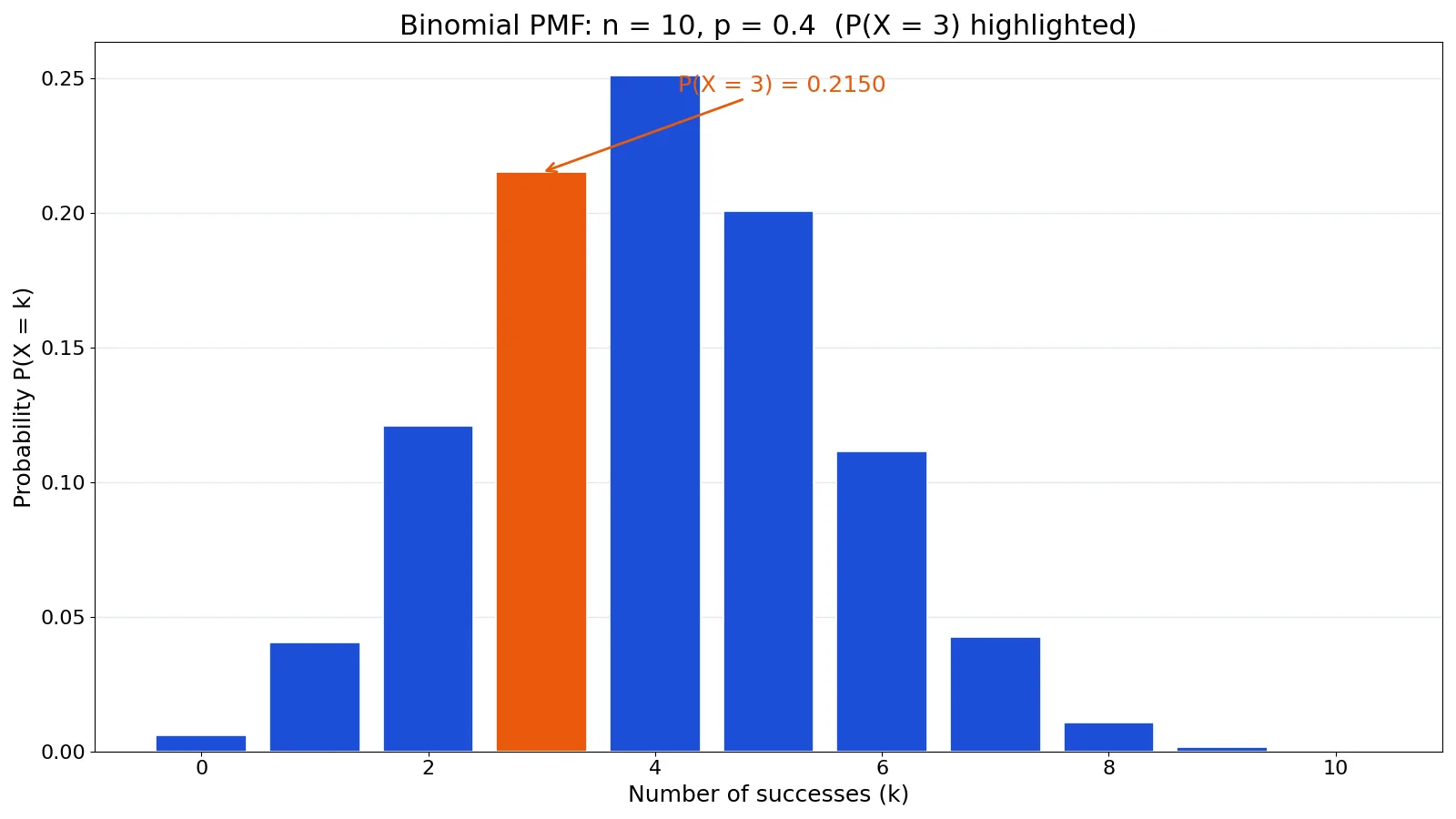
The binomial formula gives the probability of getting exactly $k$ successes in $n$ independent trials when each trial has the same success probability $p$. You plug in three numbers, $n$, $k$ and $p$, and you get a single probability. The same three numbers also give you the mean and standard deviation of the distribution.

This article covers the formula, the conditions it requires, a full worked example with real numbers, and the exact functions to use in Excel, R and Python.

Quick Answer

The binomial formula is $P(X = k) = \binom{n}{k} p^k (1-p)^{n-k}$, where $\binom{n}{k}$ counts the ways to choose which trials succeed [1].
It applies when you have a fixed number of independent trials, two outcomes per trial, and a constant success probability $p$ [1].
The mean is $\mu = np$, the variance is $\sigma^2 = np(1-p)$, and the standard deviation is $\sigma = \sqrt{np(1-p)}$ [2].
For $n = 10$, $p = 0.4$ and $k = 3$, the probability is 0.2150, the mean is 4.0000 and the standard deviation is 1.5492.
In Excel, =BINOM.DIST(3,10,0.4,FALSE) returns the same 0.2150.

The Formula

The probability mass function of the binomial distribution is [1][3]:

$$P(X = k) = \binom{n}{k} p^k (1-p)^{n-k} \quad \text{for } k = 0, 1, 2, \dots, n$$

Each symbol means something specific:

Symbol	Meaning
$n$	The fixed number of trials
$k$	The number of successes you are asking about
$p$	The probability of success on a single trial, the same for every trial [1]
$\binom{n}{k}$	The binomial coefficient, read "n choose k"
$p^k$	The probability that the $k$ successes all happen
$(1-p)^{n-k}$	The probability that the remaining $n-k$ trials all fail

The binomial coefficient is defined as [1]:

$$\binom{n}{k} = \frac{n!}{k!(n-k)!}$$

It counts how many different orderings of $k$ successes among $n$ trials exist. For example, $\binom{10}{3} = 120$, so there are 120 distinct patterns of three successes in ten trials.

The distribution has four requirements. The number of trials is fixed in advance. Each trial has exactly two mutually exclusive outcomes, usually called success and failure [1]. The trials are independent. The success probability $p$ stays constant across trials [1].

If you want the probability of $k$ or fewer successes, you sum the individual probabilities. That is the cumulative distribution function [1]:

$$F(k; p, n) = \sum_{i=0}^{k} \binom{n}{i} p^i (1-p)^{n-i}$$

How to Calculate It Step by Step

Confirm the setting is binomial. Check the four conditions above. If the trials are not independent or $p$ changes, this formula does not apply.
Write down $n$, $p$ and $k$. Be clear about which outcome counts as a success, because $p$ is defined for that outcome.
Compute the binomial coefficient $\binom{n}{k} = \frac{n!}{k!(n-k)!}$.
Compute $p^k$, the success probability raised to the number of successes.
Compute $(1-p)^{n-k}$, the failure probability raised to the number of failures.
Multiply the three pieces together. That product is $P(X = k)$.
For the mean and spread, use $\mu = np$, $\sigma^2 = np(1-p)$ and $\sigma = \sqrt{np(1-p)}$ [2].

Steps 3 to 6 are the ones people get wrong by hand, usually through a factorial slip or by mixing up $k$ and $n-k$.

Worked Example

Twelve students each run 10 independent Bernoulli trials with a success probability of 0.4, and the number of successes is recorded for each student. The question is the probability that a single student gets exactly 3 successes.

student_id	name	n_trials	p_success	successes
1	A. Rivera	10	0.4	3
2	B. Chen	10	0.4	5
3	C. Okafor	10	0.4	2
4	D. Patel	10	0.4	4
5	E. Novak	10	0.4	3
6	F. Haddad	10	0.4	6
7	G. Silva	10	0.4	1
8	H. Kim	10	0.4	4
9	I. Rossi	10	0.4	3
10	J. Muller	10	0.4	5
11	K. Tanaka	10	0.4	2
12	L. Dubois	10	0.4	4

The parameters are $n = 10$, $p = 0.4$ and $k = 3$. Working through the formula:

Step	Value
Identify parameters	n = 10, p = 0.4, k = 3
Combinations C(n,k)	C(10,3) = 120
p^k	0.4^3 = 0.064000
(1-p)^(n-k)	(1-0.4)^7 = 0.027994
PMF by hand	120 × 0.064000 × 0.027994 = 0.2150
PMF via scipy.stats.binom	binom.pmf(3, 10, 0.4) = 0.2150
Mean	n × p = 10 × 0.4 = 4.0000
Variance	n × p × (1-p) = 10 × 0.4 × 0.6 = 2.4000
Standard deviation	sqrt(2.4000) = 1.5492
Excel equivalent	=BINOM.DIST(3,10,0.4,FALSE) → 0.2150

So $P(X = 3) = 0.2150$. About 21.5% of students running this experiment would be expected to land on exactly 3 successes.

The mean of 4.0000 says the long-run average number of successes is 4. The standard deviation of 1.5492 says typical results sit roughly 1.5 successes away from that average. In the table above, the observed counts run from 1 to 6, which is consistent with a mean of 4 and that spread.

How to Interpret the Result

A single binomial probability answers a narrow question: how likely is exactly this count? That is often not what you actually want. If you ask "how likely is 3 or fewer successes," you need the cumulative probability, which sums every value from 0 to 3. The cumulative form is what most decisions use, because ranges are usually more meaningful than exact points.

The mean and standard deviation describe the whole distribution, not one outcome. For a binomial distribution, the mean $np$ is the expected count of successes if you repeated the experiment many times [2]. The standard deviation tells you how far a typical result drifts from that mean. A small standard deviation means results cluster tightly around the mean. A large one means they scatter.

One useful check: the standard deviation is largest when $p = 0.5$ and shrinks toward zero as $p$ approaches 0 or 1. That matches intuition. If success is nearly certain or nearly impossible, there is little room for variation.

Doing It in Software

Hand calculation is fine for small numbers, but factorials grow fast and rounding creeps in. Software handles the arithmetic exactly. Many calculators and programs have built-in functions for binomial coefficients, factorials and full binomial probabilities [2].

In Excel, BINOM.DIST takes the number of successes, the number of trials, the probability and a logical flag. FALSE gives the exact probability, TRUE gives the cumulative probability. For this example, =BINOM.DIST(3,10,0.4,FALSE) returns 0.2150.

In R, the dbinom function gives the probability mass, pbinom gives the cumulative probability, and qbinom gives quantiles [4]. The call dbinom(3, size = 10, prob = 0.4) returns 0.2150.

In Python, SciPy provides the same functions through scipy.stats.binom [3]:

from scipy.stats import binom
n, p, k = 10, 0.4, 3
p_exact = binom.pmf(k, n, p)   # 0.2150
mean = n * p                   # 4.0000
sd = (n * p * (1 - p)) ** 0.5  # 1.5492

Output:

P(X = 3) = 0.2150
Mean = 4.0000
Standard deviation = 1.5492

If you would rather not write code, the Binomial Distribution Calculator takes $n$, $p$ and $k$ and returns the probability, mean and standard deviation directly. The Probability Calculator is useful when you need to combine several probability results.

Common Mistakes

Using the formula when trials are not independent. Drawing cards without replacement changes $p$ on every draw, so the binomial model does not fit. Use the hypergeometric distribution instead.
Confusing $k$ with $n-k$ in the exponents. The exponent on $p$ is the number of successes, and the exponent on $(1-p)$ is the number of failures. Swapping them gives a wrong answer that still looks plausible.
Reporting the exact probability when you need a range. "Exactly 3" and "3 or fewer" are different questions. Use the cumulative function for the second one.
Forgetting that $p$ must be the probability of the outcome you call success. If you define success as the rarer outcome, $p$ is small and the mean shifts accordingly.
Assuming the mean is the most likely value. The mean $np$ is the expected count, but when $p$ is far from 0.5 the most likely single value can differ from the mean.
Rounding intermediate steps too early. Rounding $p^k$ or $(1-p)^{n-k}$ before multiplying can shift the final probability in the third decimal place.

Limitations

The binomial distribution only models a fixed number of independent trials with a constant success probability. Real data often violates one of those conditions. Trials may be correlated, the number of trials may not be fixed in advance, or $p$ may drift over time. When that happens, the binomial probabilities will be wrong, sometimes badly.

The distribution also says nothing about why successes occur. It gives you probabilities under stated assumptions, not causes. A good fit to a binomial model does not prove the underlying process is truly independent and identically distributed. It only means the model is consistent with the data you have.

For very large $n$, computing exact probabilities can be slow or numerically awkward, and the normal approximation to the binomial is often used instead [2]. That approximation works well when $np$ and $n(1-p)$ are both reasonably large, but it is an approximation, not the exact answer.

Frequently Asked Questions

What is the difference between the binomial formula and the binomial distribution?

The formula is the rule that assigns a probability to each possible number of successes. The distribution is the full set of those probabilities across every value of $k$ from 0 to $n$. The formula is one piece of the distribution.

Can the binomial formula be used for more than two outcomes?

No. The binomial model requires exactly two mutually exclusive outcomes per trial, labeled success and failure [1]. If a trial has three or more possible outcomes, you need a different model, such as the multinomial distribution.

How do I find the binomial standard deviation?

Take the square root of the variance. The variance is $np(1-p)$, so the binomial standard deviation is $\sqrt{np(1-p)}$ [2]. For $n = 10$ and $p = 0.4$, that is $\sqrt{2.4} = 1.5492$.

What does the binomial distribution in a calculator actually compute?

Most calculators and software packages offer two modes. The exact mode returns $P(X = k)$ for one value of $k$. The cumulative mode returns $P(X \le k)$, the sum of all probabilities up to and including $k$ [1]. Check which mode you are in before reading the result.

When should I use the normal approximation instead?

Use it when $n$ is large and $p$ is not too close to 0 or 1, so that both $np$ and $n(1-p)$ are comfortably large [2]. The approximation is faster but less exact, so prefer the exact binomial calculation when your software can handle it.

Is the binomial distribution the same as the Bernoulli distribution?

The Bernoulli distribution models a single trial with two outcomes. The binomial distribution models the total number of successes across $n$ independent Bernoulli trials. A binomial with $n = 1$ is a Bernoulli distribution, which is covered in the Bernoulli distribution guide.