Standard Deviation of a Binomial Distribution: Formula and Example

By Dr. Zubair Khalid, DVM, MS, PhD · 2026-10-03

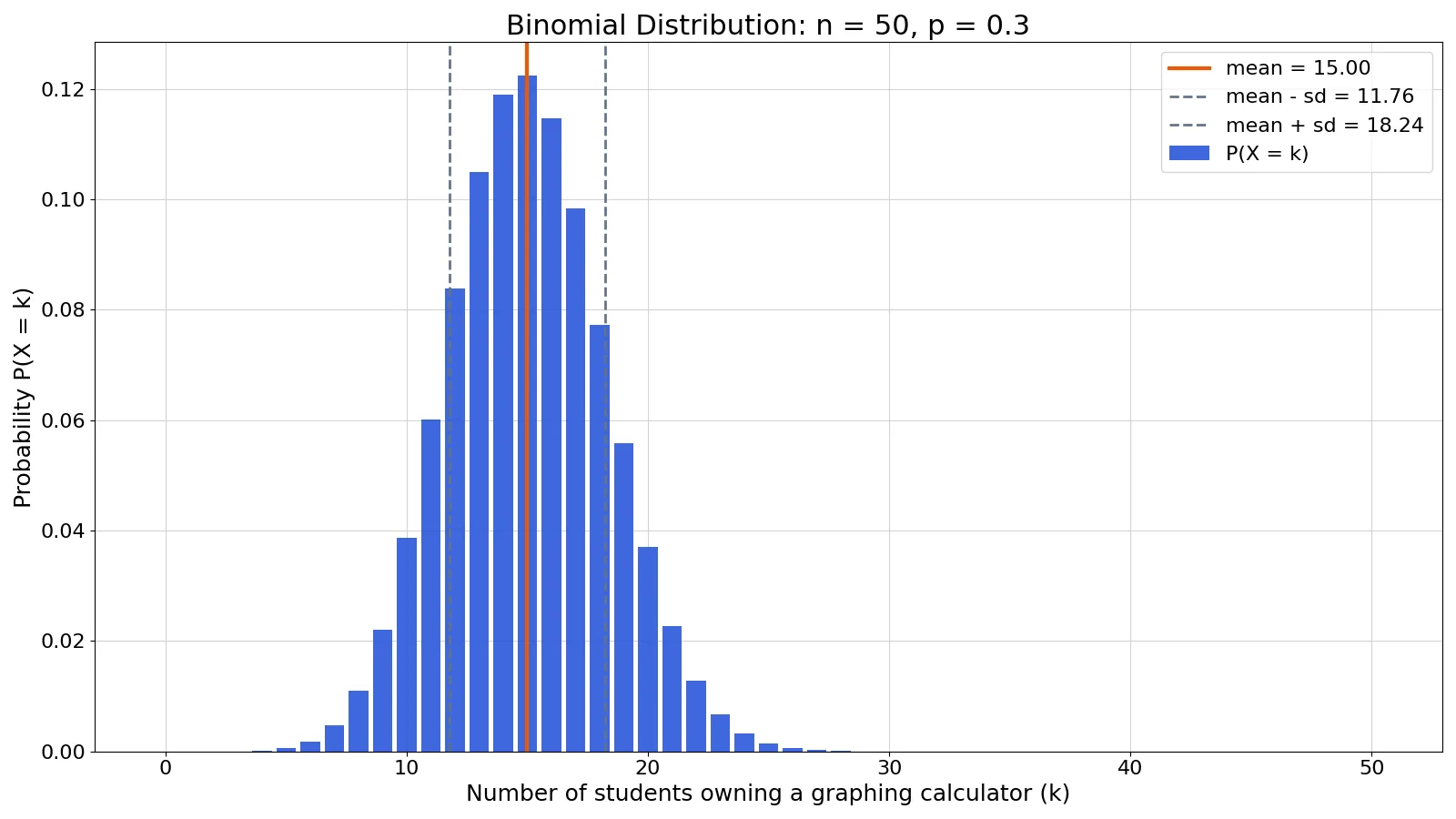
The standard deviation of a binomial distribution measures how far the number of successes typically falls from its expected value. You compute it as $\sigma = \sqrt{np(1-p)}$, where $n$ is the number of trials and $p$ is the probability of success on each trial. This article gives you the formula, a full worked example, and the software commands to reproduce it.

Quick Answer

The standard deviation of a binomial distribution is $\sigma = \sqrt{np(1-p)}$ [1].
The variance is the value under the square root, $\sigma^2 = np(1-p)$.
The mean is $\mu = np$, and the standard deviation is the square root of the variance [1].
For $n = 50$ and $p = 0.3$, the variance is 10.5000 and the standard deviation is 3.2404.
The standard deviation is in the same units as the count of successes, not in percent.

The Formula

The standard deviation of a binomial distribution is the square root of the variance:

$$\sigma = \sqrt{np(1-p)}$$

Each symbol means the following.

Symbol	Meaning
$n$	Number of independent trials
$p$	Probability of success on a single trial
$1-p$	Probability of failure on a single trial
$np$	Mean number of successes, written $\mu$
$np(1-p)$	Variance of the number of successes, written $\sigma^2$
$\sigma$	Standard deviation of the number of successes

The binomial setting requires exactly two mutually exclusive outcomes per trial, a fixed probability $p$ on every trial, and independent trials [2]. When those conditions hold, the number of successes $X$ follows a binomial distribution, and the mean and standard deviation come from the formulas above [1]. The same structure appears in the simpler Bernoulli distribution, which is the binomial case with $n = 1$.

How to Calculate It Step by Step

Confirm the setting is binomial: fixed number of trials, two outcomes, constant $p$, independent trials.
Write down $n$, the number of trials.
Write down $p$, the probability of success on one trial.
Compute the mean, $\mu = np$.
Compute the variance, $\sigma^2 = np(1-p)$.
Take the square root of the variance to get $\sigma = \sqrt{np(1-p)}$.
Round to a sensible number of decimals and report the units.

Steps 4 through 6 are the same arithmetic you use for any mean and standard deviation pair, applied to a count variable.

Worked Example

Suppose a regional survey finds that 30% of students own a graphing calculator, so $p = 0.3$. You plan to sample $n = 50$ students and count how many own one. A small pilot survey of 12 students recorded ownership as 1 for yes and 0 for no.

student_id	owns_calculator
S01	1
S02	0
S03	1
S04	0
S05	0
S06	1
S07	0
S08	0
S09	1
S10	0
S11	0
S12	1

The pilot gives 5 owners out of 12, so $\hat{p} = 5/12 = 0.4167$. That is a rough check on the assumed rate, not the value used in the formula. The calculation uses the planned parameters $n = 50$ and $p = 0.3$.

Step 1. Identify the parameters. $n = 50$, $p = 0.3$.

Step 2. Compute the mean.

$$\mu = np = 50 \times 0.3 = 15.0000$$

Step 3. Compute the variance.

$$\sigma^2 = np(1-p) = 50 \times 0.3 \times 0.7 = 10.5000$$

Step 4. Take the square root.

$$\sigma = \sqrt{np(1-p)} = \sqrt{10.5000} = 3.2404$$

So the expected number of owners is 15.0000, and the typical distance from that value is about 3.2404 students. The mean plus or minus one standard deviation runs from 11.76 to 18.24.

How to Interpret the Result

The standard deviation tells you the spread of the count, not the spread of the proportion. A value of 3.2404 means that in repeated samples of 50 students, the number of owners typically lands within about 3.24 of 15. Values near 15 are common, and values far from 15 are rare.

You can use the result to judge whether an observation is unusual. The interval from $\mu - \sigma$ to $\mu + \sigma$ is 11.76 to 18.24. An observed count of 25 owners sits well above that range, which suggests either an unusual sample or a true ownership rate higher than 0.3.

The spread also depends on $p$. For fixed $n$, the variance $np(1-p)$ is largest when $p = 0.5$ and shrinks as $p$ moves toward 0 or 1. A rare event has a small standard deviation in absolute terms, even though each success is surprising. If you need the spread of the proportion instead of the count, divide the standard deviation by $n$, which connects to the standard error of the mean.

Doing It in Software

All three tools below return the same value for $n = 50$ and $p = 0.3$.

Excel. Enter this formula in any cell:

=SQRT(50*0.3*(1-0.3))

Result: 3.2404.

Python. The math module handles the square root.

import math
n = 50
p = 0.3
mean = n * p            # 15.0000
var = n * p * (1 - p)   # 10.5000
sd = math.sqrt(var)     # 3.2404
print(f"mean = {mean:.4f}, variance = {var:.4f}, sd = {sd:.4f}")

Output:

mean = 15.0000, variance = 10.5000, sd = 3.2404

R. One line does the whole job.

sqrt(50*0.3*(1-0.3))

Result: 3.2404. R also ships the binomial distribution functions dbinom, pbinom, qbinom, and rbinom, where size is the number of trials and prob is the success probability [3]. For a quick check without code, the Binomial Distribution Calculator returns the mean and standard deviation from $n$ and $p$, and the Standard Deviation Calculator handles raw data such as the 12-student pilot.

Common Mistakes

Using the sample proportion in place of $p$. The formula needs the assumed success probability for the population, not the observed rate from your data. Fix: state $p$ from theory or prior evidence, and treat $\hat{p}$ as a separate check.
Forgetting the square root. The expression $np(1-p)$ is the variance. Fix: take the square root before you report a standard deviation.
Confusing the count with the proportion. A standard deviation of 3.2404 applies to the number of successes out of 50, not to a percentage. Fix: divide by $n$ if you want the spread of the proportion.
Applying the formula when trials are not independent. Sampling without replacement from a small population breaks independence. Fix: use the hypergeometric distribution, or confirm the population is much larger than the sample [4].
Assuming a fixed $p$ when it changes. If the success probability differs across trials, the binomial model does not apply. Fix: check that $p$ is constant before using the formula.
Reporting too many decimals. A standard deviation of 3.2404 implies precision the inputs do not support. Fix: round to two decimals, so 3.24.

Limitations

The formula only describes the spread of a count under strict binomial conditions. If trials are dependent, if $p$ varies, or if there are more than two outcomes, the result is wrong even though the arithmetic still runs. The standard deviation also says nothing about the shape of the distribution. For small $n$ or $p$ near 0 or 1, the distribution is skewed, so the mean plus or minus one standard deviation does not capture a symmetric band of probability.

The standard deviation is a summary, not a probability. It does not tell you the chance of seeing exactly 20 successes or at least 25. For those questions you need the probability mass function or the cumulative distribution function [2]. When you need tail probabilities, use the full distribution instead of the mean and standard deviation alone.

Frequently Asked Questions

What is the standard deviation of a binomial distribution?

It is $\sigma = \sqrt{np(1-p)}$, where $n$ is the number of trials and $p$ is the probability of success on each trial [1]. It measures the typical distance between the observed number of successes and the mean $np$. The value is always non-negative and is zero only when $p$ is 0 or 1.

Is the standard deviation of a binomial distribution the same as the variance?

No. The variance is $\sigma^2 = np(1-p)$, and the standard deviation is its square root. For $n = 50$ and $p = 0.3$, the variance is 10.5000 and the standard deviation is 3.2404. The standard deviation is in the same units as the count, while the variance is in squared units.

How do I find the standard deviation for a binomial distribution in Excel?

Use =SQRT(n*p*(1-p)) with your values in place of the letters. For $n = 50$ and $p = 0.3$, =SQRT(50*0.3*(1-0.3)) returns 3.2404. Excel has no single built-in function for the binomial standard deviation, so you build it from the formula.

What happens to the standard deviation when n increases?

The standard deviation grows with the square root of $n$ when $p$ is fixed. Doubling $n$ multiplies the standard deviation by about 1.414. The spread of the proportion, $\sqrt{p(1-p)/n}$, shrinks as $n$ grows, which is why larger samples give more precise estimates.

Can the standard deviation of a binomial distribution be larger than the mean?

Yes, when $1-p$ is large enough. The ratio of the standard deviation to the mean is $\sqrt{(1-p)/(np)}$, which exceeds 1 when $np(1-p) > n^2p^2$. This happens for small $n$ and small $p$, where the distribution is strongly right-skewed and most trials produce zero successes.