Exponential Distribution: Definition, Formula and Examples

By Dr. Zubair Khalid, DVM, MS, PhD · 2026-10-03

The exponential distribution is a continuous probability distribution that models the time you wait until the next event occurs, such as the next customer call, machine failure, or earthquake. It has one parameter, the rate $\lambda$, and its defining feature is a constant hazard rate, which makes it the standard model for memoryless waiting times.

Quick Answer

The exponential distribution models the waiting time between events in a Poisson process, where events happen at a constant average rate.
It has one parameter: the rate $\lambda$ (events per unit time). The mean and standard deviation both equal $1/\lambda$.
PDF: $f(x) = \lambda e^{-\lambda x}$ for $x \ge 0$. CDF: $F(x) = 1 - e^{-\lambda x}$ [1].
The tail probability is simple: $P(X > x) = e^{-\lambda x}$ [2].
It is memoryless, meaning past waiting time does not change the distribution of the remaining wait [3].

What the Exponential Distribution Means

In plain terms, the exponential distribution describes how long you wait for something to happen when it happens at a steady average rate and the timing is random. Short waits are common, long waits are rare, and the curve drops off quickly as $x$ grows [4].

The precise statistical definition: a continuous random variable $X$ follows an exponential distribution with rate parameter $\lambda > 0$ if its probability density function is

$$f(x) = \lambda e^{-\lambda x}, \quad x \ge 0$$

and $f(x) = 0$ for $x < 0$. The parameter $\lambda$ is the rate, the average number of events per unit of time. Some textbooks and software use the scale parameter $\beta = 1/\lambda$ instead, which equals the mean [1]. Both forms describe the same distribution, so always check which parameterization a tool is using.

How It Works

The exponential distribution is built from two functions. The probability density function (PDF) gives the relative likelihood of a value, and the cumulative distribution function (CDF) gives the probability of falling at or below a value.

Probability density function

$$f(x) = \lambda e^{-\lambda x}, \quad x \ge 0, \; \lambda > 0$$

Cumulative distribution function

$$F(x) = P(X \le x) = 1 - e^{-\lambda x}, \quad x \ge 0$$

Each symbol means:

$x$ is the value of the waiting time you are evaluating.
$\lambda$ (lambda) is the rate, the average number of events per unit time.
$e$ is Euler's number, about 2.71828.
$1/\lambda$ is the mean waiting time, also called the expected value $E[X]$.

The survival function, the probability of waiting longer than $x$, is the complement of the CDF:

$$P(X > x) = e^{-\lambda x}$$

For a range between two values, subtract the CDFs:

$$P(x_1 \le X \le x_2) = e^{-\lambda x_1} - e^{-\lambda x_2}$$

The mean and standard deviation are both $1/\lambda$. The median is $\ln(2)/\lambda$, which is about $0.693/\lambda$ [3]. The exponential distribution is the only continuous distribution with a constant failure rate, which is why it is central to reliability work [3]. If you want the broader family context, see probability distributions explained.

Worked Example

Suppose a call center records the waiting times, in minutes, for 20 customer service calls. The observed data are:

waiting_time_min
0.4
1.1
0.7
2.3
0.9
1.6
3.2
0.5
1.8
2.7
0.6
1.3
4.1
0.8
2.0
1.5
0.3
3.6
1.9
0.2

Assume the waiting times follow an exponential distribution with rate $\lambda = 0.5$ calls per minute. Here is the full walkthrough.

Step 1. State the rate. $\lambda = 0.5$ per minute.

Step 2. Mean waiting time. $E[X] = 1/\lambda = 1/0.5 = 2.0000$ minutes.

Step 3. Standard deviation. $SD[X] = 1/\lambda = 2.0000$ minutes.

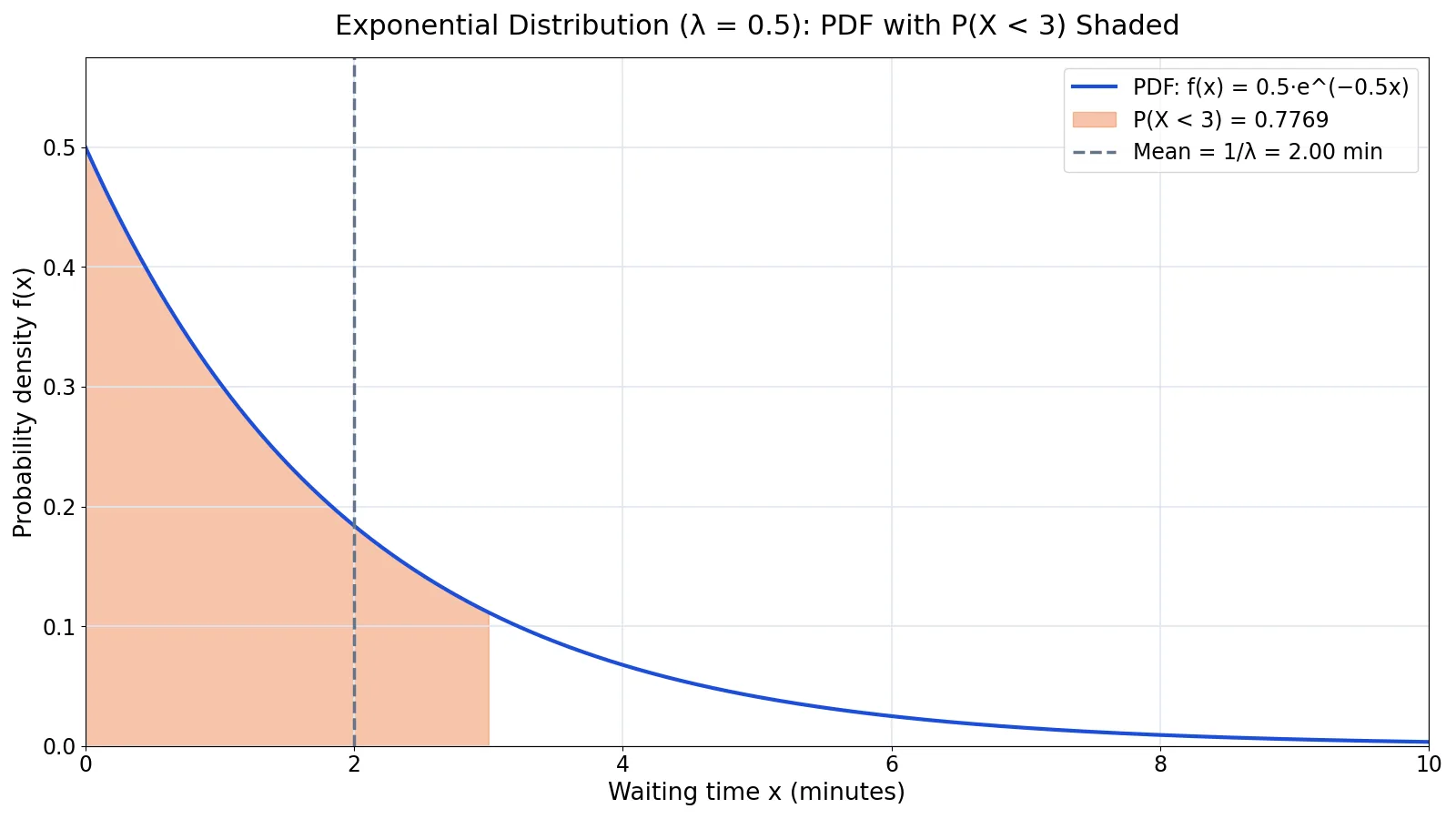
Step 4. CDF at $x = 3$. $P(X < 3) = 1 - e^{-\lambda x} = 1 - e^{-0.5 \cdot 3} = 1 - e^{-1.5000} = 0.7769$.

Step 5. Tail probability. $P(X > 3) = e^{-1.5000} = 0.2231$.

Step 6. PDF at $x = 3$. $f(3) = \lambda e^{-\lambda \cdot 3} = 0.5 \cdot e^{-1.5000} = 0.1116$.

Step 7. Compare to the sample. The observed sample mean is $\bar{x} = 1.5750$ minutes with $n = 20$, which is lower than the theoretical mean of 2.0000 minutes.

In Python, the same values come from one function call:

from scipy import stats
lam = 0.5
p_lt_3 = stats.expon.cdf(3, scale=1/lam)  # scale is 1/lambda
mean = 1/lam
print(f"P(X < 3) = {p_lt_3:.4f}; mean = {mean:.4f} minutes; P(X > 3) = {stats.expon.sf(3, scale=1/lam):.4f}")

Output:

P(X < 3) = 0.7769; mean = 2.0000 minutes; P(X > 3) = 0.2231

The shaded area under the PDF from $x = 0$ to $x = 3$ equals $P(X < 3) = 0.7769$, and the dashed line marks the mean $1/\lambda = 2.00$ minutes.

How to Interpret It

The rate $\lambda$ controls how fast the curve decays. A larger $\lambda$ means events arrive more often, so the mean wait $1/\lambda$ shrinks and the curve falls off faster. A smaller $\lambda$ stretches the distribution to the right.

The CDF value is the probability that the wait is at or below your threshold. In the example, $P(X < 3) = 0.7769$ means about 77.69% of waits are under 3 minutes. The tail value $P(X > 3) = 0.2231$ means about 22.31% of waits exceed 3 minutes. These two always sum to 1.

The PDF value is not a probability. $f(3) = 0.1116$ is a density, so it only becomes a probability when multiplied by a small interval width. To read probabilities, use the CDF or the survival function. If you want to compute $e^{-\lambda x}$ directly in a spreadsheet, the EXP function in Excel does exactly that.

When to Use It (and when not to)

Use the exponential distribution when you are modeling the time until the next event and the event rate is roughly constant. Good fits include interarrival times in a Poisson process, the lifetime of components with a constant failure rate, and the time between arrivals at a service desk [3]. It also works for the amount of time until an earthquake or the length of a phone call [4].

Do not use it when the hazard rate changes over time. If failures become more likely as a part wears out, the exponential model is wrong and a distribution with an increasing hazard rate fits better. Do not use it for a variable that can be negative, since the exponential distribution only covers $x \ge 0$. Do not use it when the data are clearly clustered around a value far from zero, which points to a different shape entirely.

Exponential Distribution vs Poisson Distribution

These two distributions describe the same process from two angles. The Poisson distribution counts how many events occur in a fixed interval, and the exponential distribution measures the time between those events [4]. If events arrive at rate $\lambda$ per unit time, the count per unit time is Poisson with mean $\lambda$, and the waiting time is exponential with rate $\lambda$ [5].

Feature	Exponential	Poisson
Variable type	Continuous (time)	Discrete (count)
Question answered	How long until the next event?	How many events in a period?
Parameter	Rate $\lambda$	Mean $\lambda$
Mean	$1/\lambda$	$\lambda$
Range	$x \ge 0$	$k = 0, 1, 2, \dots$
Typical use	Waiting times	Event counts

For the counting side, see Poisson distribution: formula and examples.

Common Mistakes

Confusing rate and mean. The parameter $\lambda$ is a rate, not the mean. The mean is $1/\lambda$. Fix: check whether your tool wants rate or scale before you plug in a number [1].
Treating the PDF value as a probability. $f(x)$ is a density and can exceed 1. Fix: use the CDF or survival function for probabilities.
Forgetting the range. The exponential distribution is defined only for $x \ge 0$. Fix: set the probability to 0 for negative values.
Assuming memorylessness always holds. Memorylessness means the remaining wait does not depend on how long you have already waited [3]. Fix: test this assumption before relying on it, since wear-out processes violate it.
Using the wrong tail. $P(X > x)$ and $P(X < x)$ are complements. Fix: compute one and subtract from 1 to get the other.
Mixing up parameterizations across software. Some tools use scale $\beta = 1/\lambda$. Fix: confirm the argument name, such as scale in SciPy, before interpreting output.

Limitations

The exponential distribution assumes a constant hazard rate, so it cannot capture processes where risk rises or falls over time. Real-world lifetimes often show wear-out or infant-mortality patterns that a single rate cannot represent. It also cannot model values below zero, and it forces the highest density at zero, which is unrealistic for variables that cluster around a positive value.

With small samples, the estimated rate can be unstable, and a single extreme observation can pull the mean noticeably. The sample mean in the worked example, 1.5750 minutes, differs from the theoretical 2.0000 minutes, which is normal sampling variation at $n = 20$. Always report the sample size alongside the estimate.

Frequently Asked Questions

What does the exponential distribution model?

It models the waiting time until the next event in a process where events occur at a constant average rate. Common examples include the time between customer arrivals, the time until a machine fails, and the length of a phone call [4]. The key requirement is that the event rate stays roughly constant over the period you study.

What is the difference between the exponential and Poisson distributions?

The Poisson distribution counts events in a fixed interval, while the exponential distribution measures the time between events. They are two views of the same process. If the count per unit time is Poisson with mean $\lambda$, the waiting time is exponential with rate $\lambda$ [5].

What is the mean of the exponential distribution?

The mean is $1/\lambda$, where $\lambda$ is the rate. The standard deviation is also $1/\lambda$, so the mean and standard deviation are equal. In the worked example with $\lambda = 0.5$ per minute, both equal 2.0000 minutes.

What does memoryless mean in the exponential distribution?

Memoryless means the remaining waiting time does not depend on how long you have already waited. If a component has survived 12 years, the probability it lasts 7 more years is the same as for a new component [5]. This property holds only for the exponential distribution among continuous distributions [3].

How do I compute exponential probabilities?

Use the CDF $F(x) = 1 - e^{-\lambda x}$ for the probability of waiting at most $x$, and the survival function $e^{-\lambda x}$ for waiting more than $x$ [2]. For a range, subtract the two CDF values. Software such as SciPy computes these directly with the rate or scale parameter.

References

1.3.6.6.7. Exponential Distribution
6.3: Exponential Distribution - Statistics LibreTexts/06%3A_Continuous_Probability_Distributions/6.03%3A_Exponential_Distribution)
8.1.6.1. Exponential
5.4: The Exponential Distribution - Statistics LibreTexts/05%3A_Continuous_Random_Variables/5.04%3A_The_Exponential_Distribution)
5.3 The Exponential Distribution (Optional) - Statistics | OpenStax