Geometric Distribution: Formula and Examples

By Dr. Zubair Khalid, DVM, MS, PhD · 2026-10-03

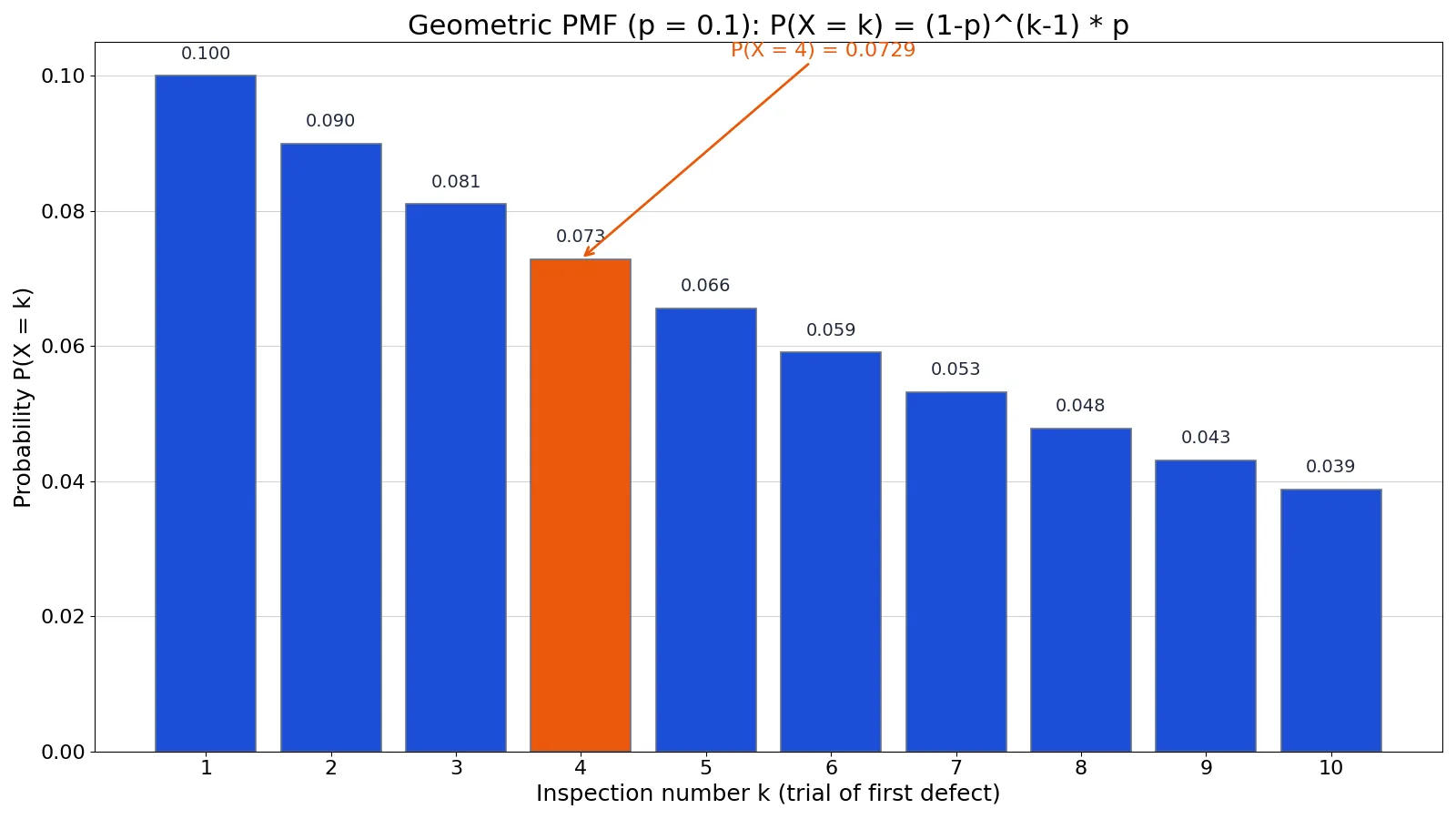
The geometric distribution models the number of trials you run until the first success in a sequence of independent trials with the same success probability. Its probability mass function is $P(X = x) = p \cdot q^{x-1}$ for $x = 1, 2, 3, \dots$, where $p$ is the success probability and $q = 1 - p$ [1]. This article gives you the formula, the assumptions behind it, and a worked example you can check line by line.

Quick Answer

The geometric distribution counts trials up to and including the first success [1].
Its PMF is $P(X = x) = p \cdot q^{x-1}$, with $q = 1 - p$ and $x = 1, 2, 3, \dots$ [1].
The mean is $\mu = 1/p$, and the variance is $\sigma^2 = (1-p)/p^2$ [2].
Trials must be independent, each with two outcomes and a constant success probability [3].
A "success" is just the event you are counting, even if it is something bad like finding a defect [1].

What the Geometric Distribution Means

In plain terms, the geometric distribution answers one question: how long do I wait until the first success? You keep running trials until the event happens, then you stop and record how many trials it took.

The precise statistical definition: if a random experiment satisfies the geometric requirements, the distribution of the random variable $X$, where $X$ counts the number of trials until the first success, is called a geometric distribution. If a discrete random variable $X$ has a geometric distribution with success probability $p$, we write $X \sim G(p)$ [1].

Two counting conventions exist. In Case I, $X$ is the number of trials including the success, so $x = 1, 2, 3, \dots$ [2]. In Case II, $X$ is the number of failures before the success, so $x = 0, 1, 2, \dots$ and the PMF is $P(X = x) = (1-p)^x p$ [2]. This article uses Case I throughout, which is the more common convention in introductory texts.

How It Works

The formula follows directly from the structure of the experiment. To get your first success on trial $x$, you need $x - 1$ failures in a row, then one success. Each failure has probability $q = 1 - p$, and the success has probability $p$.

$$P(X = x) = p \cdot q^{x-1}, \quad x = 1, 2, 3, \dots$$

Each symbol means the following:

Symbol	Meaning
$X$	Number of trials up to and including the first success
$x$	The specific trial number you are finding the probability for
$p$	Probability of success on a single trial
$q$	Probability of failure on a single trial, $q = 1 - p$

Because the trials are independent, you multiply the probabilities of the individual outcomes. That is why the formula is a product of $x - 1$ failure probabilities and one success probability [1].

The cumulative probability, the chance the first success happens by trial $k$, is:

$$P(X \le k) = 1 - q^{k}$$

The mean and standard deviation describe the long-run behavior. For Case I, the expected value is $\mu = 1/p$, which tells you how many trials to expect until the first success, counting the successful trial itself [2]. The variance is $\sigma^2 = (1-p)/p^2$, and the standard deviation is its square root [2].

Worked Example

An inspection log records 10 parts. Each part independently has a defect probability of $p = 0.1$, and the first defective part appears at inspection 4. The data look like this:

Inspection	Defective
1	0
2	0
3	0
4	1
5	0
6	0
7	0
8	0
9	0
10	0

Here a "success" is finding a defect, which is not a good thing, but it is the event being counted [1]. The steps are:

Assumptions. Independent trials, constant success probability $p$, count trials until the first success.
Parameter. $p = 0.1$.
Failure probability. $q = 1 - 0.1 = 0.9000$.
PMF formula. $P(X = 4) = (0.9000)^{4-1} \cdot 0.1$.
Compute the power. $(0.9000)^3 = 0.7290$.
Multiply by $p$. $0.7290 \cdot 0.1 = 0.0729$.
CDF. $P(X \le 4) = 0.3439$.
Mean. $1 / 0.1 = 10.0000$.
Variance. $(0.9000) / (0.1)^2 = 90.0000$.
Standard deviation. $\sqrt{90.0000} = 9.4868$.

So the probability that the first defect lands exactly on inspection 4 is 0.0729, and the probability it appears by inspection 4 is 0.3439. On average you would expect the first defect around inspection 10, with a standard deviation of about 9.49 inspections.

You can reproduce these numbers in Python:

from scipy.stats import geom
p = 0.1
k = 4
pmf = geom.pmf(k, p)   # 0.0729
cdf = geom.cdf(k, p)   # 0.3439
mean = 1 / p           # 10.0000
print(f"pmf = {pmf:.4f}\ncdf = {cdf:.4f}\nmean = {mean:.4f}")

Output:

pmf = 0.0729
cdf = 0.3439
mean = 10.0000

How to Interpret It

The PMF value 0.0729 is a probability for one specific trial number. It does not mean 7.29 percent of parts are defective. It means that if you repeated this inspection process many times, about 7.29 percent of those runs would see their first defect on the fourth part.

The CDF value 0.3439 is cumulative. It says roughly a third of inspection runs would find a defect within the first four parts. The remaining two thirds would need more than four inspections.

The mean of 10 is a long-run average, not a prediction for any single run. With $p = 0.1$, the distribution is heavily right skewed, so most runs end early while a few run very long. That skew is why the standard deviation of 9.49 is almost as large as the mean itself. For a broader look at this shape, see right skewed distribution examples.

When to Use It (and when not to)

Use the geometric distribution when all of these hold [3]:

Each trial has exactly two outcomes, success or failure.
The trials are independent of one another.
The probability of success $p$ stays the same on every trial.
You are counting trials until the first success, then stopping.

Typical uses include quality control sampling until the first defect, counting coin flips until the first head, and modeling how many attempts a process needs before it succeeds.

Do not use it when the probability changes between trials, when trials influence each other, or when you are counting successes across a fixed number of trials. That last case belongs to the binomial distribution, which fixes the number of trials and lets the number of successes vary. If you are counting how many trials it takes to reach a fixed number of successes, you want the negative binomial distribution instead.

Geometric Distribution vs Binomial Distribution

Both distributions rest on independent trials with a constant success probability. The difference is what you hold fixed and what you count.

Feature	Geometric	Binomial
What is fixed	Number of successes (one)	Number of trials
What varies	Number of trials	Number of successes
Possible values	$x = 1, 2, 3, \dots$	$x = 0, 1, \dots, n$
PMF	$p \cdot q^{x-1}$	$\binom{n}{x} p^x q^{n-x}$
Mean	$1/p$	$np$
Typical question	How many trials until the first success?	How many successes in $n$ trials?

If you already know the number of trials and want a count of successes, switch to the binomial model. If the number of trials is the unknown, the geometric model fits. For a wider view of how these families relate, see probability distributions explained.

Common Mistakes

Confusing the two counting conventions. Case I counts the success trial, Case II counts only failures before it. The PMFs differ by a factor of $q$. Fix: state up front whether $x$ starts at 1 or 0, and keep it consistent.
Using $x = 0$ with the Case I formula. The formula $p \cdot q^{x-1}$ requires $x \ge 1$. Fix: if your data can show zero failures before the success, use the Case II form $(1-p)^x p$ [2].
Treating "success" as something good. A success is simply the event you are counting, and it can be a defect or a crash [1]. Fix: define the success event in words before you assign $p$.
Assuming a fixed $p$ when it drifts. If the defect rate rises as a machine wears down, the constant-$p$ assumption fails. Fix: check the process for stability, or use a model that allows a changing probability.
Reading the mean as a guarantee. A mean of 10 does not mean the first success arrives at trial 10. Fix: report the spread alongside the mean, since the standard deviation can be large.
Ignoring independence. Sampling without replacement from a small batch makes trials dependent. Fix: confirm independence, or use a model built for sampling without replacement.

Limitations

The geometric distribution assumes a constant success probability and independent trials. Real processes often violate both. A machine that degrades, a user who learns from each attempt, or a batch sampled without replacement all break the assumptions, and the formula will misstate the probabilities.

The distribution also describes only the wait for the first success. It says nothing about the second, third, or later successes, and it cannot handle more than two outcomes per trial. When you need counts of multiple successes or more than two categories, another model is the right tool. For a refresher on the building blocks, see fundamental statistics core concepts.

Frequently Asked Questions

What is the geometric distribution formula?

The formula is $P(X = x) = p \cdot q^{x-1}$ for $x = 1, 2, 3, \dots$, where $p$ is the probability of success on one trial and $q = 1 - p$ is the probability of failure [1]. It gives the probability that the first success occurs on trial $x$. A second form, $P(X = x) = (1-p)^x p$ for $x = 0, 1, 2, \dots$, counts failures before the success instead [2].

What are the assumptions of the geometric distribution?

Each trial must have two possible outcomes, the trials must be independent, and the probability of success must stay the same on every trial [3]. You also stop as soon as the first success occurs. When these conditions hold, the number of trials up to and including the first success follows a geometric distribution [1].

What is the mean of a geometric distribution?

For the trial-counting form, the mean is $\mu = 1/p$ [2]. With $p = 0.1$, the mean is 10 trials. This value counts the successful trial itself, so it is the expected number of trials until the first success, not the expected number of failures.

What is the difference between geometric and binomial distribution?

The binomial distribution fixes the number of trials and counts the successes. The geometric distribution fixes the number of successes at one and counts the trials needed to reach it. Both require independent trials with a constant success probability, so the assumptions overlap even though the questions differ.

Can the geometric distribution be used for more than two outcomes?

No. It requires exactly two outcomes per trial, typically labeled success and failure. If your experiment has three or more categories, you need a different model. You can sometimes collapse categories into two groups, but that changes the meaning of $p$ and should be done deliberately.

If you are comparing candidate models for count data, the Poisson distribution is worth checking alongside the geometric, since both describe counts but under different assumptions.

References

4.3: Geometric Distributions - Statistics LibreTexts
4.4 Geometric Distribution - Introductory Statistics 2e | OpenStax
5.3: Geometric Distributions - Statistics LibreTexts/05%3A_Discrete_Probability_Distributions/5.03%3A_Geometric_Distributions)