How to Sum a Column in Excel (Step by Step)

By Dr. Zubair Khalid, DVM, MS, PhD · 2026-10-03

Knowing how to sum a column in Excel is one of the first skills that makes a spreadsheet useful. You can total a column with AutoSum in a couple of clicks, type a SUM formula yourself, or just select the cells and read the total off the status bar. This guide covers all three, plus the errors that trip people up.

Quick Answer

AutoSum: select the empty cell below your numbers, go to Home > AutoSum, then press Enter. Excel proposes a range and totals it.
SUM function: type =SUM(B2:B16) in any empty cell and press Enter. Replace the range with your own column.
Status bar: select the cells you want to add and read the sum in the status bar at the bottom of the window. No formula is created.
Running total: use a mixed reference such as =SUM($B$2:B2) and copy it down the column.
Check the range: AutoSum guesses which cells to include, so confirm the highlighted range before you press Enter.

Before You Start

A few things decide which method works best.

First, check that your numbers are really numbers. Text that looks like a number, such as a value typed with a leading apostrophe or imported as text, will be ignored by SUM. If a total looks too low, this is the usual cause.

Second, leave the cell directly below your data empty. AutoSum looks upward from the active cell and stops at the first blank row or non-numeric cell, so a gap in the middle of your column can cut the range short.

Third, decide whether you want a static total or a live one. A formula updates when the source numbers change. A status bar reading does not, because it is only a display.

If you are new to writing formulas at all, start with how to make a formula in Excel and come back here.

Step by Step

Method 1: AutoSum

Click the empty cell directly below the column you want to total. In the example below, that is B17.
Go to Home > AutoSum. You can also press Alt+= as a shortcut for the same command.
Excel highlights the range it plans to add, such as B2:B16. Check that the highlight covers every row you want.
Press Enter. The total appears in the cell.

If the highlighted range is wrong, drag over the correct cells before pressing Enter, or type the range directly.

Method 2: The SUM function

Click any empty cell.
Type =SUM( and then select the cells you want to add, or type the range by hand.
Close the bracket and press Enter.

For a column of values in B2 through B16, the formula is:

=SUM(B2:B16)

The colon means "everything from B2 to B16 inclusive." Parentheses group the argument so Excel knows exactly what to add [1]. For a deeper look at the function's arguments, see Excel SUM Function: Syntax, Examples and Tips.

Method 3: Status bar total

Select the cells you want to add, for example B2:B16.
Look at the status bar at the bottom of the Excel window. It shows the sum of the selected cells.

This creates no formula and changes nothing in the sheet. It is the fastest way to check a total without editing anything.

Method 4: A running total

A running total shows the cumulative sum after each row. Enter this in the first data row and copy it down:

=SUM($B$2:B2)

The dollar signs lock the start of the range at B2 while the end moves down as you copy. Row 3 becomes =SUM($B$2:B3), row 4 becomes =SUM($B$2:B4), and so on.

Worked Example

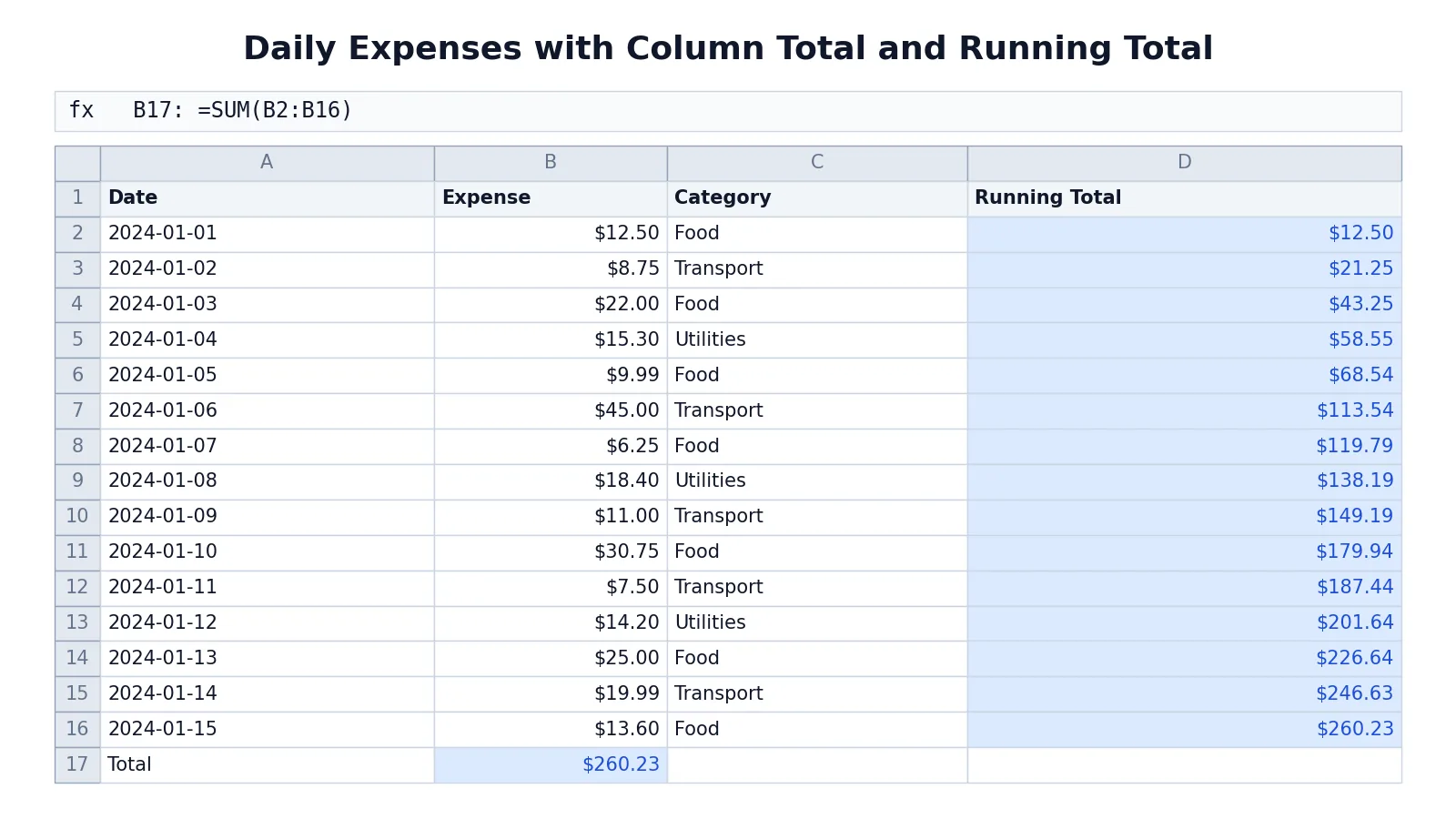
The table below is a 15-day expense log with a Date column, an Expense column, a Category column, and a Running Total column. The Expense column holds the amounts, and the Running Total column adds them up row by row.

Row	A: Date	B: Expense	C: Category	D: Running Total
1	Date	Expense	Category	Running Total
2	2024-01-01	12.5	Food	`=SUM($B$2:B2)` -> displays $12.50
3	2024-01-02	8.75	Transport	`=SUM($B$2:B3)` -> displays $21.25
4	2024-01-03	22	Food	`=SUM($B$2:B4)` -> displays $43.25
5	2024-01-04	15.3	Utilities	`=SUM($B$2:B5)` -> displays $58.55
6	2024-01-05	9.99	Food	`=SUM($B$2:B6)` -> displays $68.54
7	2024-01-06	45	Transport	`=SUM($B$2:B7)` -> displays $113.54
8	2024-01-07	6.25	Food	`=SUM($B$2:B8)` -> displays $119.79
9	2024-01-08	18.4	Utilities	`=SUM($B$2:B9)` -> displays $138.19
10	2024-01-09	11	Transport	`=SUM($B$2:B10)` -> displays $149.19
11	2024-01-10	30.75	Food	`=SUM($B$2:B11)` -> displays $179.94
12	2024-01-11	7.5	Transport	`=SUM($B$2:B12)` -> displays $187.44
13	2024-01-12	14.2	Utilities	`=SUM($B$2:B13)` -> displays $201.64
14	2024-01-13	25	Food	`=SUM($B$2:B14)` -> displays $226.64
15	2024-01-14	19.99	Transport	`=SUM($B$2:B15)` -> displays $246.63
16	2024-01-15	13.6	Food	`=SUM($B$2:B16)` -> displays $260.23
17	Total	`=SUM(B2:B16)` -> displays $260.23

Two things are worth noticing. The grand total in B17 equals the last running total in D16, which is $260.23. That agreement is a useful check that both formulas cover the same rows.

The running total formula is a common building block for trend analysis. Once you have it, you can chart the column to see how spending accumulates over the period. If you want to group the same data by category instead, a pivot table will total each group in a few clicks.

Other Ways to Do It

Sum several columns at once. Select the empty cells below each column, then use AutoSum. Excel fills each selected cell with a SUM formula for the column above it.

Sum a whole column. =SUM(B:B) adds every number in column B. It is convenient, but it also picks up any numbers you add later anywhere in that column, including subtotals, which can double-count.

Sum non-adjacent ranges. Separate each range with a comma inside the parentheses, for example =SUM(B2:B16, D2:D16).

Sum with a condition. If you only want the Food rows, use SUMIF with the category column as the criteria range.

Use a table. If you convert your range to an Excel table, the total row gives you a dropdown with Sum, Average, Count and other options. The formula updates automatically as rows are added.

Troubleshooting

The total is lower than expected. Some cells are stored as text. Select the column and check the status bar. If the count of numeric cells is smaller than the number of rows, text values are hiding in there. Re-enter them as numbers or convert the column.

The total shows 0. Either the range is wrong or every value in it is text. Click the formula cell and check the highlighted range.

The formula shows as text. The cell is formatted as Text, or the formula is missing its leading equals sign. Format the cell as General and retype the formula.

AutoSum picked the wrong range. It stopped at a blank row or a text cell. Type the range manually instead.

The total changes when you sort. This usually means the formula references fixed rows while the data moved. Use a full-column reference or a table to avoid it. See how to sort a column in Excel for the sorting steps.

A circular reference warning appears. The formula is inside the range it is summing. Move it below the data.

Common Mistakes

Including the total row in the range. If B17 holds the total, =SUM(B2:B17) counts it twice. Sum only the data rows, B2:B16.
Leaving gaps in the column. A blank cell breaks AutoSum's guess. Keep the data contiguous or type the range.
Summing a column that contains subtotals. The grand total then adds the subtotals on top of the detail rows. Remove or exclude them.
Assuming the status bar total is saved. It is a display only. If you need the number in the sheet, write a formula.
Forgetting the dollar signs in a running total. Without $B$2, copying the formula down shifts the start of the range and the running total breaks.
Mixing text and numbers in one column. SUM ignores text silently, so the total looks plausible but is wrong.

Limitations

SUM adds numbers. It cannot tell you whether the numbers are correct, whether rows are duplicated, or whether a category was mislabeled. A column that sums to $260.23 can still contain a $45 expense filed under the wrong category.

The status bar total is also easy to misread. It reflects whatever is selected at that moment, so a partial selection gives a partial total with no warning. For anything you plan to reuse, put the total in a cell as a formula so the range is visible and auditable.

Frequently Asked Questions

How do I sum a column in Excel without a formula?

Select the cells you want to add and read the total in the status bar at the bottom of the window. Nothing is written to the sheet. If you need the number to stay in the file, use AutoSum or a SUM formula instead.

Why does my SUM formula return 0?

The most common cause is that the values are stored as text, so SUM finds nothing numeric to add. Another cause is a range that points at empty cells. Check the highlighted range when you edit the formula, and confirm the cells are numbers by selecting them and watching the status bar count.

How do I add up a column in Excel that keeps growing?

Convert the range to an Excel table, then use the total row. The formula expands automatically as you add rows. A full-column reference such as =SUM(B:B) also works, but it will include any subtotal rows you add later in that column.

What is the difference between AutoSum and the SUM function?

They produce the same result. AutoSum is a command that writes a SUM formula for you after guessing the range. Typing SUM yourself gives you full control over which cells are included, which matters when the column has gaps or subtotals.

Can I sum only the visible rows after filtering?

SUM adds hidden rows too, so a filtered column will not give you the visible total. Use SUBTOTAL or AGGREGATE, which can ignore hidden rows, when you need a total that respects a filter.

References

Altman DG, Bland JM (2011). Brackets (parentheses) in formulas. BMJ

References

Further Reading
- Broman KW, Woo KH (2018). Data Organization in Spreadsheets. The American Statistician
- Ziemann M, Eren Y, El-Osta A (2016). Gene name errors are widespread in the scientific literature. Genome Biology
- Microsoft Support: Excel help and learning
- McCullough B, Heiser DA (2008). On the accuracy of statistical procedures in Microsoft Excel 2007. Computational Statistics & Data Analysis
- Abeysooriya M, Soria M, Kasu MS et al. (2021). Gene name errors: Lessons not learned. PLOS Computational Biology