Excel SUM Function: Syntax, Examples and Tips

By Dr. Zubair Khalid, DVM, MS, PhD · 2026-10-03

The Excel SUM function adds numbers from cells, ranges or typed values and returns a single total. It is the standard way to total a column in Excel because =SUM(B2:B7) is shorter and less error-prone than typing =B2+B3+B4+B5+B6+B7 [1]. This article covers the syntax, a worked example, common errors and the limits you should know about.

Quick Answer

What it does: adds numbers from individual values, cell references, ranges or a mix of all three [2].
Basic form: =SUM(number1,[number2],...) where each argument is a range, a number or a single cell reference separated by commas [1].
Typical use: =SUM(B2:B7) totals six months of sales in one step.
Fastest entry: select the cell below a column of numbers and use AutoSum, which writes the SUM formula for you [3].
Watch out for: text that looks like a number, hidden rows and blank cells inside a range.

Syntax

Argument	Required?	Meaning
number1	Yes	The first value to add. It can be a number like 4, a cell reference like B6, or a range like B2:B8 [2].
number2, ...	No	Additional values to add. You can specify up to 255 numbers this way [2].

The general form is:

$$=\text{SUM}(number1,\ [number2],\ \dots)$$

Each argument can be a range, a number, or a single cell reference, all separated by commas [1]. A formula can mix types, for example =SUM(A2:A4,C2:C3) adds two separate ranges in one call [1].

How It Works

SUM walks through every argument you give it, pulls out the numeric values and adds them. Text values that look like numbers are translated into numbers first, and the logical value TRUE is translated into 1 [1]. So =SUM("5",15,TRUE) returns 21 because "5" becomes 5 and TRUE becomes 1 [1].

Ranges are read cell by cell. If a cell inside the range holds text, SUM ignores it and keeps going. That behavior is convenient for headers, but it also hides data-entry mistakes, which is why the errors section below matters.

You can also use negative values to subtract inside a SUM call. The formula =SUM(12,5,-3,8,-4) adds 12, subtracts 3, adds 8 and subtracts 4 in that order [4]. Excel has no SUBTRACT function, so a minus sign inside SUM or a plain minus operator is the standard approach [4].

For a column of adjacent numbers, AutoSum is the quickest route. Select the cell immediately below the last number, choose AutoSum on the Home tab, and press Enter. Excel writes the formula and highlights the cells it plans to total [3]. AutoSum also works horizontally if you select the cell to the right of a row of numbers [3]. The AutoSum Wizard detects the range automatically, and you can adjust the selection with Shift plus the arrow keys before pressing Enter [5]. It works best on contiguous ranges, and if there is a blank row or column inside the range, the selection stops at the first gap [5].

Worked Example

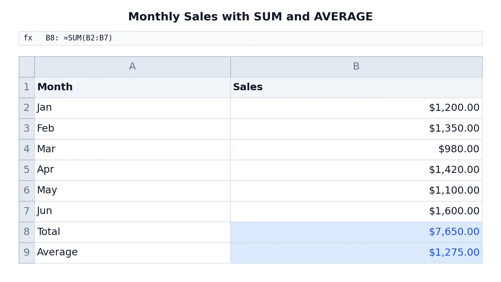
The table below holds six months of sales figures for one product line. The Total row uses SUM and the Average row uses AVERAGE on the same range.

	A	B
1	Month	Sales
2	Jan	1200
3	Feb	1350
4	Mar	980
5	Apr	1420
6	May	1100
7	Jun	1600
8	Total	`=SUM(B2:B7)` -> displays $7,650.00
9	Average	`=AVERAGE(B2:B7)` -> displays $1,275.00

Cell B8 adds all monthly sales in the range B2:B7 to get the half-year total. Cell B9 calculates the average monthly sales across the same range. The two formulas share one range reference, so if you correct a monthly figure, both the total and the average update at once.

If you later add a July row, insert it above row 8 so the range expands to B2:B8. Inserting a row directly above the Total row is the safe habit because SUM picks up the new row automatically.

More Examples

Two ranges in one formula. =SUM(A2:A4,C2:C3) adds the numbers in ranges A2:A4 and C2:C3 and returns their combined total [1]. This is useful when the columns you need are not next to each other.

A range plus a constant. =SUM(A2:A4,15) adds the values in cells A2 through A4 and then adds 15 to that result [1].

Typed values only. =SUM(12,5,-3,8,-4) returns 18. The minus signs subtract the third and fifth values [4].

Mixed types. =SUM("5",15,TRUE) returns 21 because the text "5" is converted to 5 and TRUE is converted to 1 [1].

Summing time values. If you are adding hours and minutes and want the result to display that way, =SUM(A6:C6) gives the total hours and minutes without multiplying by 24 [2].

Summing only visible cells. When you hide rows manually or filter a list, SUM still includes the hidden values. Use the SUBTOTAL function instead if you want only the visible cells totaled [2]. SUBTOTAL(9,...) skips rows hidden by a filter, and SUBTOTAL(109,...) also skips rows you hid manually. A total row in an Excel table behaves the same way, because any function you pick from the Total drop-down is entered as a subtotal [2].

Conditional totals. When you need to add only the values that meet a condition, such as total sales for one product, use SUMIF and SUMIFS instead of plain SUM [6]. For totals that involve multiplying matching arrays, see the SUMPRODUCT function.

Errors and How to Fix Them

The total is too low and a cell shows a green triangle. That cell holds text that looks like a number, so SUM skipped it. Convert the cell to a number or retype the value.

The result is 0 when you expect a total. The range probably points at the wrong column, or every cell in it is text. Click the formula and check the highlighted range on the sheet.

#VALUE! appears. One of your arguments is text that cannot be converted to a number, such as a word typed directly into the formula. Remove that argument or point it at a numeric cell.

The formula shows as text instead of calculating. The cell is formatted as Text, or the formula was typed with a leading apostrophe. Set the cell format to General and re-enter the formula.

The total does not change when you filter. SUM includes hidden rows, so a filtered total looks wrong. Switch to SUBTOTAL for visible-only totals [2].

Common Mistakes

Typing every cell instead of a range. =A2+A3+A4+A5+A6 breaks the moment a row is inserted. Use =SUM(A2:A6), which is less likely to contain typing errors [1].
Leaving a blank row inside the range. AutoSum stops at the first gap, so the formula may cover only part of your data [5]. Check the highlighted range before pressing Enter, or build the formula by hand.
Assuming SUM ignores hidden rows. It does not. Hidden and filtered rows are still counted, so use SUBTOTAL when you need visible-only totals [2].
Mixing text and numbers in one column. SUM quietly skips the text, so the total looks plausible but is wrong. Keep numeric columns numeric.
Forgetting that TRUE counts as 1. Logical values inside a SUM argument are converted to numbers [1]. If a cell holds TRUE, it adds 1 to your total.
Using SUM where a condition is needed. Plain SUM cannot filter by product, region or date. Reach for SUMIF or SUMIFS for one or more conditions [6].

Limitations

SUM adds whatever numeric values sit in the range you give it. It cannot apply conditions, ignore hidden rows, or tell you that a value is missing. If a month is blank because the data was never entered, the total simply comes out lower with no warning. Conditional totals need SUMIF or SUMIFS, and visible-only totals need SUBTOTAL [2][6].

SUM also has no built-in error handling. If any cell in the range contains an error value, the whole formula returns that error. You have to fix or exclude the bad cell first. For large models, that means SUM is best treated as a straightforward arithmetic tool, with data validation and pivot tables doing the checking work around it.

Frequently Asked Questions

How do I total a column in Excel quickly?

Select the cell immediately below the last number in the column, choose AutoSum on the Home tab, and press Enter. Excel writes a SUM formula and highlights the cells it plans to total [3]. You can also find AutoSum under the Formulas tab [3].

What is the difference between SUM and AutoSum?

AutoSum is a feature that writes a SUM formula for you. The SUM function is the formula itself. AutoSum detects the range automatically and builds the formula, so you only need to confirm it with Enter [5][4].

Why does my SUM formula return 0?

The most common cause is that the cells contain text rather than numbers, so SUM finds nothing to add. Check the cell format and look for a green triangle in the corner of the cells. Another cause is a range that points at the wrong column.

Does SUM include hidden or filtered rows?

Yes. SUM counts hidden rows and rows excluded by a filter. If you want a total of only the visible cells, use the SUBTOTAL function instead [2]. In an Excel table, functions chosen from the Total drop-down are entered as subtotals for the same reason [2].

Can I add numbers in different columns with one SUM formula?

Yes. Separate each range with a comma, as in =SUM(A2:A4,C2:C3), which adds the values in both ranges [1]. You can include up to 255 number arguments in a single SUM formula [2].

If you need to count entries rather than add them, the COUNT function is the matching tool. For rounding a total before you report it, see the ROUND function.