How to Unhide Columns in Excel (Step by Step)

By Dr. Zubair Khalid, DVM, MS, PhD · 2026-10-03

If you need to know how to unhide columns in Excel, the fastest method is to select the columns on both sides of the hidden one, right-click the selected headers, and choose Unhide. A double line between two column headers is the visual clue that a column is hidden there [1]. The only tricky case is column A, because there is no column to its left to select.

Quick Answer

Select the headers on both sides of the hidden column, right-click, and pick Unhide [1].
You can also double-click the double line between the two headers where the hidden column sits [1].
To reveal every hidden column at once, click the Select All button and use Home > Format > Hide & Unhide > Unhide Columns.
If column A is hidden, type A1 in the Name Box, press Enter, then use Home > Format > Hide & Unhide > Unhide Columns [2].
Hidden columns are not printed in Excel for the web, so unhide them before you print [3].

Before You Start

Two things make this task easier. First, learn to spot a hidden column. Excel shows a double line between the two column headers that surround the hidden column, and the header letters skip a value [1]. If you see A, C, D, then B is hidden.

Second, decide whether you want to reveal one column or all of them. Selecting the whole sheet and choosing Unhide Columns restores every hidden column in the worksheet, which may be more than you want [2]. If you only need one column back, select just the neighbors.

If you are working with a sheet where rows are also missing, the same logic applies to rows, and you can follow the steps in How to Unhide Rows in Excel alongside this guide.

Step by Step

Look at the column headers and find the gap. A missing letter or a double line marks the hidden column [1].
Click the column header to the left of the hidden column and drag to the header on the right, or click the left header and Shift+click the right one, so the selection spans the hidden column [1].
Right-click either selected header.
Choose Unhide from the menu [1].
Check that the column reappears and that any formulas in it recalculate.

For the special case where column A is hidden, there is no left neighbor. Use the Name Box instead.

In the Name Box next to the formula bar, type A1 and press Enter [2].
Go to Home > Format.
Under Visibility, point to Hide & Unhide, then select Unhide Columns [2].

You can also right-click the column B header and pick Unhide Columns to bring back column A [2].

If you want to reveal everything at once, click the Select All button at the top-left corner of the sheet, the gray square where row 1 and column A meet. Then go to Home > Format > Hide & Unhide > Unhide Columns.

Worked Example

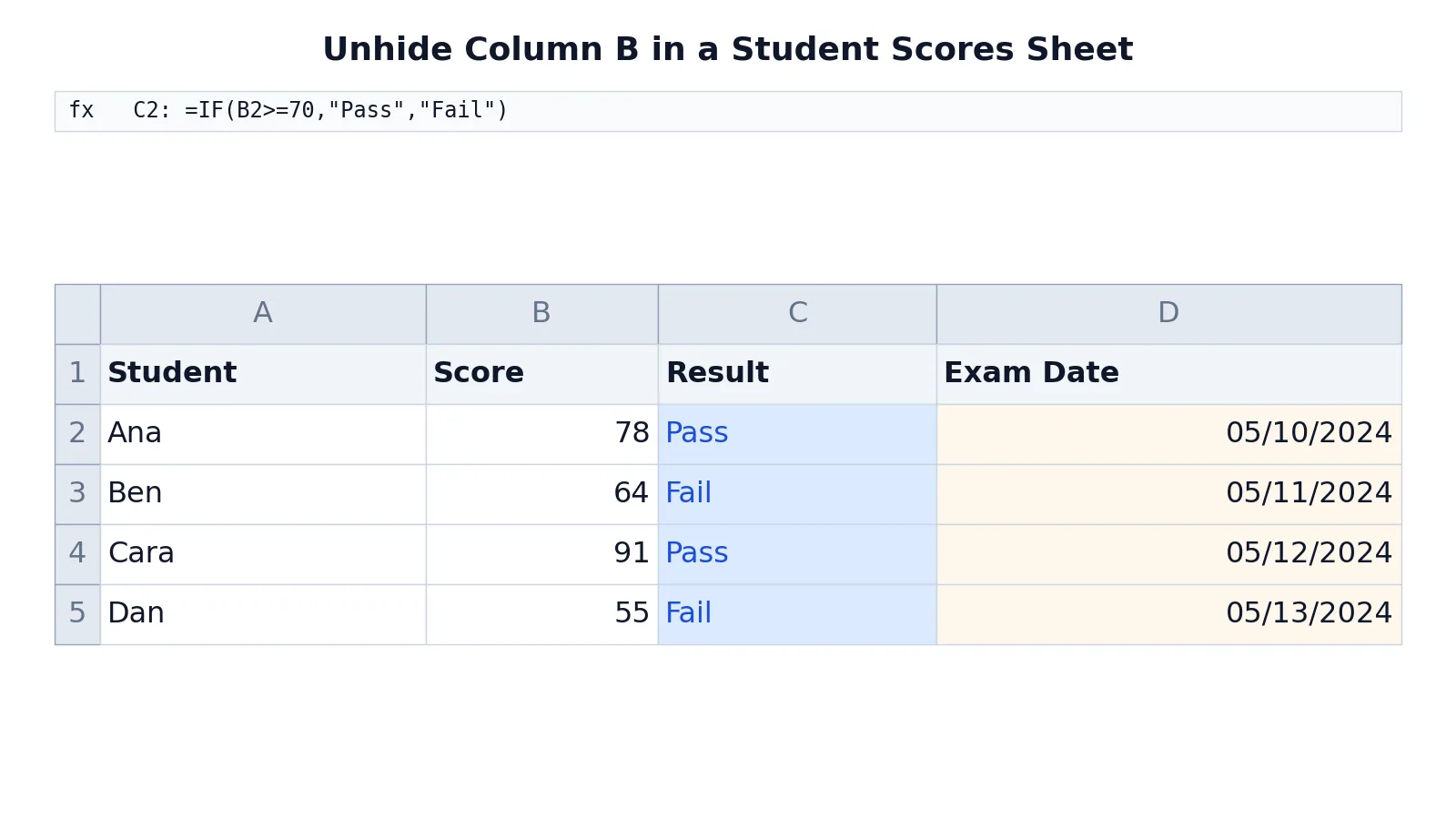
Here is a small grade sheet with four students. Column B holds the scores, column C holds a formula that checks each score, and column D holds exam dates.

	A	B	C	D
1	Student	Score	Result	Exam Date
2	Ana	78	`=IF(B2>=70,"Pass","Fail")` -> displays Pass	`=DATE(2024,5,10)` -> displays 05/10/2024
3	Ben	64	`=IF(B3>=70,"Pass","Fail")` -> displays Fail	`=DATE(2024,5,11)` -> displays 05/11/2024
4	Cara	91	`=IF(B4>=70,"Pass","Fail")` -> displays Pass	`=DATE(2024,5,12)` -> displays 05/12/2024
5	Dan	55	`=IF(B5>=70,"Pass","Fail")` -> displays Fail	`=DATE(2024,5,13)` -> displays 05/13/2024

Each Result cell runs the same test. The formula in C2 checks Ana's score and returns Pass or Fail, C3 checks Ben's score, C4 checks Cara's score, and C5 checks Dan's score. The logic is:

$$ \text{Result} = \begin{cases} \text{Pass} & \text{if Score} \ge 70 \\ \text{Fail} & \text{if Score} < 70 \end{cases} $$

Now hide column B. The headers jump from A to C, and a double line appears between them [1]. The Result column still shows Pass, Fail, Pass, Fail because the formulas keep reading the hidden scores. To bring the scores back, select columns A and C, right-click, and choose Unhide. The Score values reappear and the Result formulas recalculate to the same values.

If you had hidden column A instead, the Name Box method would be the way back. Type A1, press Enter, then use Home > Format > Hide & Unhide > Unhide Columns [2].

Other Ways to Do It

The right-click method is the quickest for a single column. Two other routes work well.

The ribbon route: select the surrounding columns, then go to Home > Format, point to Hide & Unhide, and select Unhide Columns [2]. This is the same command you use for the column A case.

The double-click route: when you see the double line between two headers, double-click it and the hidden column returns [1]. This is handy when you only have one hidden column and want to avoid the menu.

If you plan to hide and show columns often, it helps to understand the reverse action too. The same menu holds the Hide command, and the steps are covered in the related guides on hiding and showing data.

Troubleshooting

The Unhide option is grayed out. You probably have not selected the right headers. Select the columns on both sides of the hidden one, then right-click again [1].

Column A is still missing. The Name Box method is the reliable fix. Type A1, press Enter, then use Home > Format > Hide & Unhide > Unhide Columns [2].

You cannot find the hidden column. Use Find & Select > Go To Special, choose Visible cells only, and click OK. The borders of rows and columns next to hidden ones appear with a white border, which helps you locate them [4]. This feature is not available in Excel for the web [4].

The column comes back but the data looks wrong. Check the formulas. A hidden column still calculates, so unhiding it should not change results unless the formula references something that moved.

You want to unhide everything. Click Select All, then use Home > Format > Hide & Unhide > Unhide Columns. Remember this reveals every hidden column in the sheet, and hidden rows need Unhide Rows separately [2].

Common Mistakes

Selecting only one neighbor column. Excel needs a selection that spans the hidden column. Fix: drag across both neighbor headers [1].
Trying to right-click column A when it is hidden. There is no header to click. Fix: use the Name Box and type A1 [2].
Using Select All when you only want one column back. This reveals every hidden column in the sheet [2]. Fix: select just the surrounding headers.
Forgetting that hidden columns still calculate. A hidden Score column still feeds the Result formulas. Fix: unhide before you audit or print the sheet.
Printing without unhiding. In Excel for the web, hidden rows and columns are not printed [3]. Fix: unhide them before you print [3].
Confusing a narrow column with a hidden one. A very narrow column still shows its header letter. Fix: look for the missing letter or the double line [1].

Limitations

Unhiding columns only changes what you see. It does not recover deleted data, and it does not fix a column that was removed with Delete instead of Hide. If the header letter is gone and there is no double line, the column was deleted, not hidden.

The Select All method reveals every hidden column at once, which can clutter a sheet you had carefully trimmed for printing or review [2]. The Go To Special trick for locating hidden cells is not available in Excel for the web [4], so browser users have fewer options. If you are preparing a sheet for others, unhide and then re-hide only what you need.

Frequently Asked Questions

How can I unhide column A in Excel?

Type A1 in the Name Box next to the formula bar and press Enter. Then go to Home > Format, point to Hide & Unhide, and select Unhide Columns [2]. You can also right-click the column B header and pick Unhide Columns [2].

How do I unhide columns in Excel without right-clicking?

Select the surrounding column headers, then use Home > Format > Hide & Unhide > Unhide Columns [2]. You can also double-click the double line between the two headers where the hidden column sits [1].

How do I hide a column in Excel?

Select the column header, right-click it, and choose Hide [1]. To hide several nonadjacent columns, hold Ctrl as you select each header, then right-click and choose Hide [1].

Why is my Unhide option grayed out?

The command needs the headers on both sides of the hidden column to be selected. Select the left and right neighbors, then right-click again [1]. If column A is hidden, use the Name Box method instead [2].

Does unhiding a column change my formulas?

No. A hidden column still calculates normally, so the values do not change when you unhide it. In the worked example, the Result formulas returned Pass, Fail, Pass, Fail whether or not the Score column was visible.