How to Find the Mean From a Histogram (With Examples)

By Dr. Zubair Khalid, DVM, MS, PhD · 2026-10-03

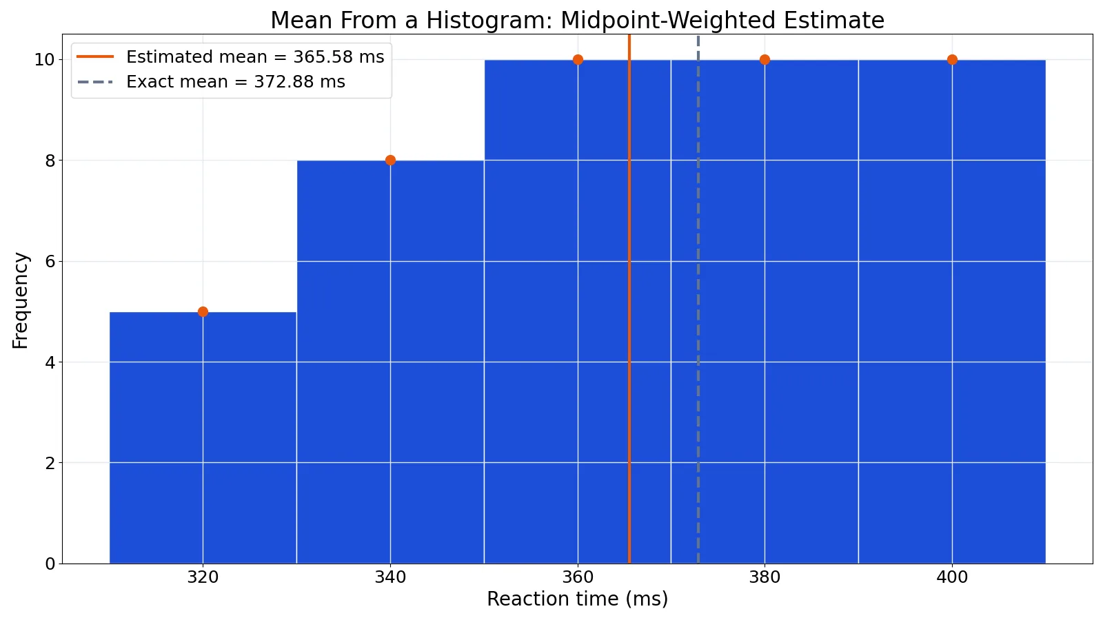
To find the mean from a histogram, multiply each class midpoint by its frequency, add those products, and divide by the total number of observations. The histogram gives you the frequencies from the bar heights, and the class midpoints stand in for the individual values you no longer have. The result is an estimate of the mean, not the exact mean, because every value in a class is represented by the same midpoint.

Quick Answer

Read each bar's height to get the frequency $f$ for that class.
Find each class midpoint $m$ by averaging the lower and upper class limits.
Multiply each midpoint by its frequency to get $f \times m$.
Add all the $f \times m$ products to get $\sum f m$.
Divide by the total frequency $n$: $\bar{x} \approx \dfrac{\sum f m}{n}$.

Before You Start

You need three things from the histogram: the class intervals, the frequency of each class, and the total count. The class intervals are usually printed along the horizontal axis. The frequencies come from the bar heights, which you read off the vertical axis. If the vertical axis shows relative frequencies instead of counts, the bar height is the count in a class divided by the total number of observations, so you will need to convert back to counts before using the formula below [1].

The midpoint formula does not require equal class widths, but equal widths are the normal case for a histogram. Narrower classes make the midpoint a closer stand-in for the values inside each class. If your classes have different widths, the midpoint method still works, but you should double-check that the bars were drawn on a consistent scale.

One more thing to confirm: whether the class limits are inclusive or exclusive. A bin labeled 310-330 usually means values from 310 up to but not including 330, so the midpoint is 320. Small differences here rarely change the answer much, but consistency matters.

If you want to compute the mean of the raw values instead, see How to Calculate the Mean: Formula and Step by Step Examples.

Step by Step

List the classes and their frequencies. Write each class interval in one column and the frequency from the bar height in the next. Add the frequencies to get $n$, the total number of observations.

Compute each class midpoint. For a class with lower limit $L$ and upper limit $U$:

$$m = \frac{L + U}{2}$$

For the class 310-330, the midpoint is $(310 + 330) / 2 = 320$.

Multiply midpoint by frequency. For each class, compute $f \times m$. This treats all $f$ observations in that class as if they sat exactly at the midpoint.

Sum the products. Add every $f \times m$ value to get $\sum f m$.

Divide by the total frequency. The estimated mean is:

$$\bar{x} \approx \frac{\sum f m}{n}$$

Sanity-check the result. The estimated mean should fall inside the range of the data and usually near the tallest bars. If it lands outside the smallest and largest class midpoints, you made an arithmetic error.

Worked Example

The dataset is 50 reaction times in milliseconds, grouped into five 20-ms bins. After grouping, 43 observations fall inside the five bins shown, so $n = 43$.

Bin label	Lower	Upper	Midpoint $m$	Frequency $f$	$f \times m$
310-330	310	330	320	5	1600
330-350	330	350	340	8	2720
350-370	350	370	360	10	3600
370-390	370	390	380	10	3800
390-410	390	410	400	10	4000

The midpoints are 320, 340, 360, 380, and 400. The frequencies are 5, 8, 10, 10, and 10. The products $f \times m$ are 1600, 2720, 3600, 3800, and 4000.

Add the products:

$$\sum f m = 1600 + 2720 + 3600 + 3800 + 4000 = 15720$$

Divide by the total frequency:

$$\bar{x} \approx \frac{15720}{43} = 365.5814 \text{ ms}$$

So the estimated mean reaction time is about 365.58 ms. The exact mean of the 50 raw values is 372.88 ms, a difference of about 7.30 ms. Part of that gap comes from grouping, because every value is moved to its bin midpoint. Part comes from the 7 raw values that fall outside the plotted bins and are left out of the estimate entirely, so the two means do not describe the same set of observations.

Here is the same calculation in Python, using numpy.histogram to get the counts and then applying the midpoint formula.

import numpy as np
raw = [...]  # 50 reaction times
bins = [310, 330, 350, 370, 390, 410]
counts, _ = np.histogram(raw, bins=bins)
mid = [(bins[i]+bins[i+1])/2 for i in range(len(bins)-1)]
est = sum(c*m for c, m in zip(counts, mid)) / counts.sum()
print(round(est, 4))  # 365.5814

Output:

365.5814

If you want to check the arithmetic by hand, a Mean, Median & Mode Calculator will confirm the division step.

Other Ways to Do It

Spreadsheet formula. In Excel, put the midpoints in one column and the frequencies in the next. Use SUMPRODUCT for the numerator and SUM for the denominator. The formula =SUMPRODUCT(midpoints, frequencies)/SUM(frequencies) returns the estimated mean in one cell. The walkthrough in How to Calculate the Mean in Excel (Step by Step) covers the setup.

From a frequency table. If you already have a grouped frequency table, you do not need the picture at all. The histogram is just a visual version of that table, so the arithmetic is identical. See Sample Mean: Definition, Formula and Examples for how the same idea works with ungrouped data.

When you have the raw values. If the original observations are available, compute the mean directly and skip the midpoint estimate. The grouped estimate is only a substitute for data you cannot access. How to Find a Point Estimate: Formula and Examples explains when an estimate like this is the right tool.

If you need the median instead. The median from a histogram uses cumulative frequencies and interpolation inside the median class, which is a different procedure. How to Find the Median from a Histogram (Step by Step) walks through it.

Troubleshooting

The frequencies do not add up to the stated sample size. Some observations may fall outside the plotted bins, or a bar may have been misread. Recheck the vertical axis scale before trusting the result.

The vertical axis shows proportions. Convert each bar height back to a count by multiplying by the total number of observations, then proceed. A histogram normalized so the area equals one is meant for density comparisons, not for counting [1].

The classes have unequal widths. The midpoint method still gives a usable estimate, but the histogram bars are no longer directly comparable by height. Check how the chart was built before interpreting the shape.

The answer looks too far from the tallest bars. This usually means a midpoint or product was copied wrong. Recompute the $f \times m$ column one row at a time.

Common Mistakes

Using the class limits instead of the midpoints. The formula needs $m$, not $L$ or $U$. Fix: average the two limits for every class before multiplying.
Dividing by the number of classes. The denominator is the total frequency $n$, not the count of bars. Fix: sum the frequency column and use that.
Reading bar heights off the wrong axis. If the vertical axis is a proportion or a density, the height is not a count. Fix: confirm the axis label and convert if needed [1].
Forgetting that the answer is an estimate. The midpoint method assumes all values in a class sit at the center. Fix: report it as an estimate and, when possible, compare it with the mean of the raw data.
Mixing up which column is which. Swapping midpoints and frequencies produces a meaningless number. Fix: label the columns clearly before you start.
Rounding midpoints too early. Rounding each midpoint to a whole number before multiplying adds error. Fix: keep full precision until the final division.

Limitations

The midpoint estimate cannot recover information the grouping destroyed. Every observation in a class is treated as identical, so the estimate ignores the spread within classes. In the worked example, the estimate was 365.58 ms against an exact mean of 372.88 ms, a gap of about 7.30 ms. Some of that gap comes from values clustering toward one end of their bins, and some from the 7 values outside the plotted bins that the estimate never sees.

The method also says nothing about variability. You get a single number for the center, not a standard deviation, a confidence interval, or a sense of how skewed the data are. If you need those, work from the raw values. And if the bins are very wide, the estimate can be off by a lot, so treat it as a rough summary and not a precise measurement.

Frequently Asked Questions

How do you find the mean from a histogram?

Read the frequency of each bar from its height, compute the midpoint of each class, multiply each midpoint by its frequency, add the products, and divide by the total frequency. The formula is $\bar{x} \approx \sum f m / n$. The result estimates the mean of the underlying data.

Can you find the exact mean from a histogram?

No. A histogram groups values into classes, so the individual observations are no longer visible. The midpoint method gives an estimate that is usually close but rarely exact. If you have the raw data, compute the mean directly for the exact value.

What if the histogram shows relative frequencies?

Multiply each bar height by the total number of observations to recover the counts, then apply the midpoint formula. A relative histogram normalizes counts so they sum to one, which makes the bar height a proportion instead of a count [1].

Why is my histogram mean different from the mean of the raw data?

Grouping replaces every value with its class midpoint. If the data are skewed or clustered within classes, that substitution shifts the estimate. In the reaction time example, the estimate was 365.58 ms and the exact mean was 372.88 ms, partly because 7 of the 50 values fall outside the plotted bins.

Does the mean have to fall inside the tallest bar?

No. The mean depends on all the bars, not just the tallest one. It will usually sit near the center of mass of the distribution, which can be to the left or right of the tallest bar when the data are skewed.

References

1.3.3.14. Histogram