How to Calculate the Mean of a Discrete Probability Distribution

By Dr. Zubair Khalid, DVM, MS, PhD · 2026-10-03

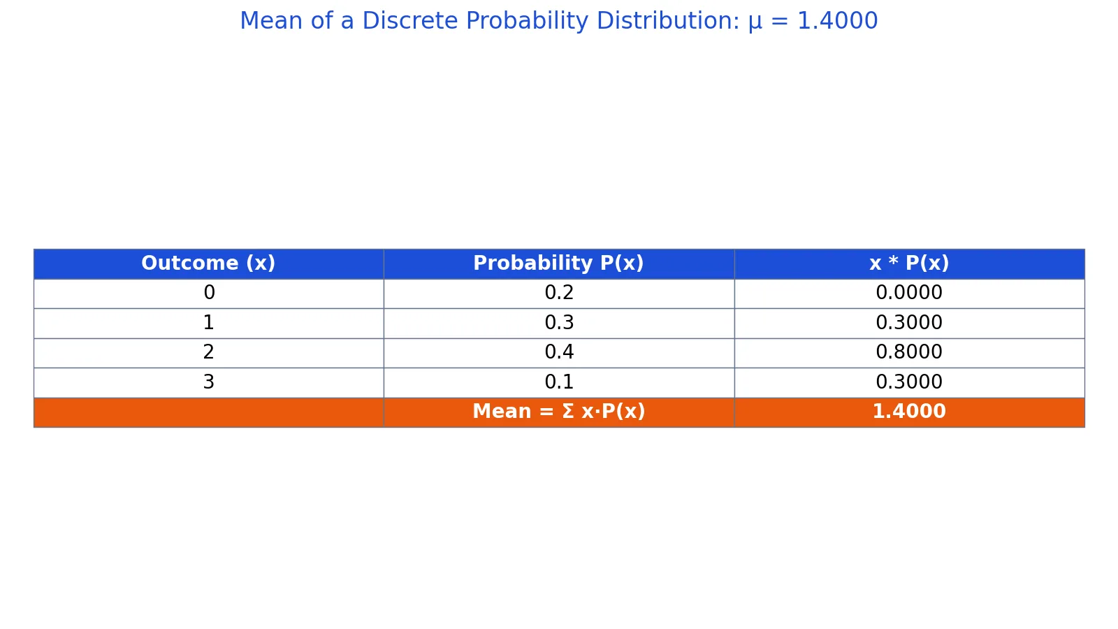
To calculate the mean for the discrete probability distribution shown here, multiply each outcome by its probability, then add those products. The result is the expected value, written $E(X)$ or $\mu$. It is the long-run average outcome if you repeated the random process many times.

Quick Answer

The mean of a discrete distribution is $\mu = \sum x \cdot P(x)$.
Multiply every outcome by its own probability. Do not multiply outcomes by each other.
Add all the products. That sum is the mean.
The mean does not have to be one of the possible outcomes. A mean of 1.4 is fine even if the outcomes are 0, 1, 2, 3.
The probabilities must sum to 1 before you start, or the answer is wrong [1].

The Formula

$$\mu = E(X) = \sum_{i} x_i \cdot P(x_i)$$

Each symbol means the following:

Symbol	Meaning
$\mu$	The mean of the distribution, also called the expected value
$E(X)$	Another name for the mean, read as "the expected value of X"
$x_i$	One possible outcome of the random variable
$P(x_i)$	The probability that outcome $x_i$ occurs
$\sum$	Sum over every possible outcome

The formula is a weighted average. Each outcome is weighted by how likely it is. Outcomes with large probabilities pull the mean toward them [2]. This is the same idea behind any weighted mean, just with probabilities as the weights.

Two conditions must hold for a valid discrete distribution. Each probability is between 0 and 1, and the probabilities over all outcomes sum to exactly 1 [1]. If your table fails either check, fix the table before computing the mean.

How to Calculate It Step by Step

List every possible outcome in one column and its probability in the next column.
Check that the probabilities sum to 1. If they do not, the table is incomplete or has an error.
Multiply each outcome by its probability. Write the product in a third column.
Add all the products from step 3.
Label the total as the mean, $\mu$ or $E(X)$.

If you want a refresher on weighted averages before starting, see how to calculate the mean.

Worked Example

The dataset is a payout distribution with four possible outcomes and their probabilities.

Outcome $x$	Probability $P(x)$	$x \cdot P(x)$
0	0.2	0.0000
1	0.3	0.3000
2	0.4	0.8000
3	0.1	0.3000

The probabilities sum to $0.2 + 0.3 + 0.4 + 0.1 = 1.0$, so the table is valid.

Now multiply each outcome by its probability:

$x = 0$, $P(x) = 0.2$: $0 \times 0.2 = 0.0000$
$x = 1$, $P(x) = 0.3$: $1 \times 0.3 = 0.3000$
$x = 2$, $P(x) = 0.4$: $2 \times 0.4 = 0.8000$
$x = 3$, $P(x) = 0.1$: $3 \times 0.1 = 0.3000$

Add the products:

$$0.0000 + 0.3000 + 0.8000 + 0.3000 = 1.4000$$

The mean is 1.4000. The outcome 2 has the largest probability, so the mean sits closer to 2 than to 0. It still lands between outcomes, which is normal for an expected value.

Here is the same calculation in Python:

outcomes = [0, 1, 2, 3]
probs = [0.2, 0.3, 0.4, 0.1]
mean = sum(x*p for x, p in zip(outcomes, probs))
print(f"{mean:.4f}")  # 1.4000

Output:

1.4000

How to Interpret the Result

The mean is the balance point of the distribution. If you ran the random process thousands of times and averaged the outcomes, the average would settle near 1.4000. It is not a prediction of any single result. One trial will give 0, 1, 2 or 3, never 1.4.

The mean also tells you the direction of the distribution. If the mean is below the midpoint of the outcome range, the distribution leans toward the smaller outcomes. If it is above the midpoint, it leans toward the larger ones. In the example, the outcomes run from 0 to 3, so the midpoint is 1.5. The mean of 1.4 sits just below it, which matches the fact that 0.2 of the probability sits at 0.

The mean alone does not describe spread. Two distributions can share a mean of 1.4 while one is tightly clustered and the other is widely scattered. Pair the mean with the standard deviation for a fuller picture, as covered in mean and standard deviation.

Doing It in Software

Excel. Put outcomes in one column and probabilities in the next. The function SUMPRODUCT multiplies matching entries and adds the results in one step. If outcomes are in A2:A5 and probabilities in B2:B5, the formula is =SUMPRODUCT(A2:A5,B2:B5). It returns 1.4 for this data. For a full walkthrough, see how to calculate the mean in Excel.

Python. The snippet above uses only built-in functions. With NumPy you can write np.sum(np.array(outcomes) * np.array(probs)), which gives the same 1.4000.

R. The expression sum(outcomes * probs) returns 1.4 when the two vectors hold the outcomes and probabilities.

For a quick check on any distribution, the probability calculator handles expected values and related probabilities without manual arithmetic.

Common Mistakes

Multiplying outcomes by each other. The formula pairs each outcome with its probability, never with another outcome. Fix: keep one product column, one row per outcome.
Using raw counts instead of probabilities. If your table shows frequencies, divide each frequency by the total first. Fix: convert to probabilities, then confirm they sum to 1.
Forgetting an outcome. A missing row changes the sum. Fix: check that the probabilities add to exactly 1 before multiplying.
Rounding too early. Rounding each product before adding can shift the final mean. Fix: keep full precision in the products and round only the final answer.
Treating the mean as a possible outcome. The mean can fall between outcomes. Fix: report it as a long-run average, not a predicted single result.
Confusing the mean with the mode. The mode is the most likely outcome. The mean is the weighted average. Fix: use the formula when you need the expected value.

Limitations

The mean summarizes center only. It says nothing about how spread out the outcomes are, so two very different distributions can share the same mean. Report the standard deviation alongside it when spread matters. The mean can also be misleading when the distribution is strongly skewed, because a few extreme outcomes pull it away from where most of the probability sits.

The method applies to discrete distributions with a finite or countable list of outcomes and known probabilities. If the probabilities are estimated from a small sample, the computed mean inherits that sampling error. If the outcome list is incomplete or the probabilities do not sum to 1, the result is not a valid expected value [1]. For continuous variables, you replace the sum with an integral, which is a different calculation, described in probability density function.

Frequently Asked Questions

What is the difference between the mean and the expected value?

They are the same quantity for a probability distribution. The expected value is the formal name, written $E(X)$, and the mean is the everyday name, written $\mu$. Both come from the same formula, $\sum x \cdot P(x)$ [2].

Can the mean be a value that is not in the table?

Yes. The mean is a weighted average, so it can fall between outcomes. In the worked example the outcomes are 0, 1, 2 and 3, but the mean is 1.4000. That value is not a possible single result.

What if the probabilities do not add up to 1?

Then the table is not a valid probability distribution. Either an outcome is missing or a probability is wrong. Fix the table first, because the mean formula assumes the probabilities cover every outcome and sum to 1 [1].

How is this different from a binomial distribution mean?

A binomial distribution is a special discrete distribution with a shortcut formula, $\mu = n \cdot p$, where $n$ is the number of trials and $p$ is the success probability. The general $\sum x \cdot P(x)$ formula still works, but the shortcut is faster. See binomial distribution for the details.

Does the mean tell me the most likely outcome?

No. The most likely outcome is the mode, the value with the highest probability. In the worked example the mode is 2, since $P(2) = 0.4$ is the largest probability, while the mean is 1.4000. Use the mean for long-run averages and the mode for single-trial predictions.

References

1.3.6.1. What is a Probability Distribution
7.3: Discrete Random Variables (3 of 5) - Chemistry LibreTexts/07%3A_6-_Probability_and_Probability_Distributions/7.03%3A_Discrete_Random_Variables_(3_of_5))