Gaussian Function: Definition, Formula and Examples

By Dr. Zubair Khalid, DVM, MS, PhD · 2026-10-03

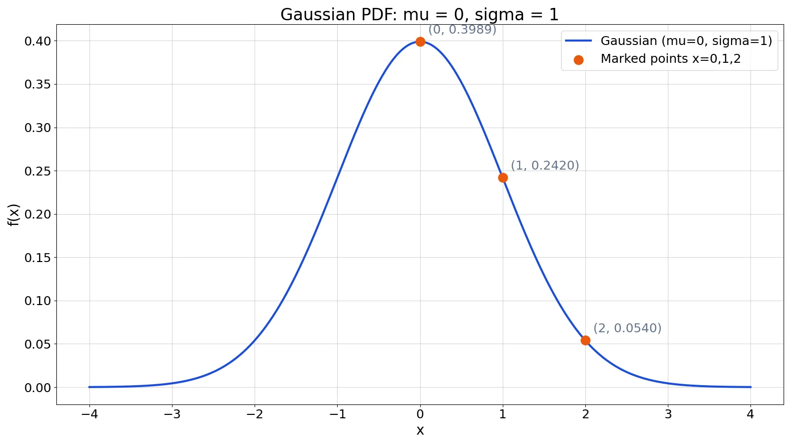
The Gaussian function is a symmetric, bell-shaped curve defined by a mean and a standard deviation. It gives the height of the curve at any value of $x$, and its shape is the basis of the normal distribution used throughout statistics [1]. This article covers the formula, a step-by-step calculation, and how to plot the curve.

Quick Answer

The Gaussian function is $f(x) = \frac{1}{\sigma\sqrt{2\pi}} e^{-\frac{(x-\mu)^2}{2\sigma^2}}$, where $\mu$ is the mean and $\sigma$ is the standard deviation.
It is also called the normal distribution or the bell curve [1].
The peak sits at $x = \mu$, and the curve is symmetric around that point.
The standard deviation controls the width. A larger $\sigma$ gives a wider, flatter curve [2].
The total area under the curve equals 1, so it works as a probability density function.

The Formula

The Gaussian probability density function is:

$$f(x) = \frac{1}{\sigma\sqrt{2\pi}} \, e^{-\frac{(x-\mu)^2}{2\sigma^2}}$$

Each symbol has a specific role:

Symbol	Meaning
$f(x)$	Height of the curve at value $x$
$x$	The value you are evaluating
$\mu$	Mean, the center of the peak
$\sigma$	Standard deviation, the spread
$\sigma^2$	Variance
$e$	Euler's number, about 2.71828
$\pi$	Pi, about 3.14159

The term $\frac{1}{\sigma\sqrt{2\pi}}$ is the normalization constant. It scales the curve so the total area under it is exactly 1 [3]. The exponential term $e^{-\frac{(x-\mu)^2}{2\sigma^2}}$ controls the shape. As $x$ moves away from $\mu$, the squared distance grows and the exponential shrinks toward zero.

This structure is closely related to the probability density function, which describes how probability is spread over a continuous range.

How to Calculate It Step by Step

Write down $\mu$ and $\sigma$ for your data.
Pick the value of $x$ you want to evaluate.
Compute the z-score: $z = \frac{x - \mu}{\sigma}$.
Square the z-score and multiply by $-0.5$.
Take $e$ raised to that result.
Multiply by the normalization constant $\frac{1}{\sigma\sqrt{2\pi}}$.

The result is the height of the curve at $x$. It is a density, not a probability, so it can be greater than 1 when $\sigma$ is small.

Worked Example

The context is a small class of 12 students and their quiz scores. The scores are shown below.

student_id	score
1	72
2	78
3	81
4	85
5	88
6	90
7	92
8	95
9	68
10	74
11	83
12	87

The mean of these scores is 82.75 and the standard deviation is 8.3897. For the calculation below, we use the standard normal case with $\mu = 0$ and $\sigma = 1$, which is the reference curve for all Gaussian functions.

Step 1. The normalization constant:

$$1/(1.0000 \times \sqrt{2\pi}) = 0.3989$$

Step 2. For $x = 0$, the z-score is $(0 - 0.0000) / 1.0000 = 0.0000$.

Step 3. The exponential term is $\exp(-0.5 \times (0.0000)^2) = 1.0000$.

Step 4. Multiply: $0.3989 \times 1.0000 = 0.3989$. This is $f(0)$.

Step 5. For $x = 1$, the z-score is $(1 - 0.0000) / 1.0000 = 1.0000$. The exponential term is $\exp(-0.5 \times (1.0000)^2) = 0.6065$. Multiply: $0.3989 \times 0.6065 = 0.2420$.

Step 6. For $x = 2$, the z-score is $(2 - 0.0000) / 1.0000 = 2.0000$. The exponential term is $\exp(-0.5 \times (2.0000)^2) = 0.1353$. Multiply: $0.3989 \times 0.1353 = 0.0540$.

The table summarizes the results.

$x$	z-score	exp term	$f(x)$	scipy value
0	0.0000	1.0000	0.3989	0.3989
1	1.0000	0.6065	0.2420	0.2420
2	2.0000	0.1353	0.0540	0.0540

The values from the hand formula match the values from scipy.stats.norm.pdf exactly.

How to Interpret the Result

The value $f(x)$ is the height of the curve, not the probability of getting exactly $x$. For a continuous distribution, the probability of any single point is zero. Probability comes from the area under the curve between two values.

For a standard normal curve, about 68.3% of the area falls within one standard deviation of the mean [1]. That means roughly two-thirds of values sit between $\mu - \sigma$ and $\mu + \sigma$. About 95% falls within two standard deviations.

In the quiz example, the mean is 82.75 and the standard deviation is 8.3897. One standard deviation covers roughly 74.4 to 91.1. Most of the class falls in that band.

The standard deviation also relates to the width of the peak. The standard deviation corresponds to the half width of the peak at about 60% of the full height [2]. A related measure you may see in the literature is the full width at half maximum, or FWHM.

Doing It in Software

Python with NumPy and SciPy is the most direct route. The snippet below computes the Gaussian by hand and compares it to the library function.

import numpy as np
from scipy.stats import norm
mu, sigma = 0.0, 1.0
for x in [0, 1, 2]:
    f = (1/(sigma*np.sqrt(2*np.pi))) * np.exp(-0.5*((x-mu)/sigma)**2)
    print(x, round(f, 4), round(norm.pdf(x, mu, sigma), 4))

Output:

0 0.3989 0.3989
1 0.242 0.242
2 0.054 0.054

In Excel, NORM.DIST(x, mean, standard_dev, FALSE) returns the density value, and NORM.DIST(x, mean, standard_dev, TRUE) returns the cumulative probability. In R, dnorm(x, mean, sd) gives the density and pnorm(x, mean, sd) gives the cumulative probability.

To plot the bell curve, generate a range of $x$ values, compute $f(x)$ for each, and draw a line chart. The curve peaks at $\mu$ and tapers off on both sides.

Common Mistakes

Treating $f(x)$ as a probability. The density can exceed 1. The fix is to integrate over an interval, or use the cumulative distribution function for a probability.
Confusing variance and standard deviation. The formula uses $\sigma$, not $\sigma^2$. The fix is to take the square root of the variance before plugging it in.
Forgetting the normalization constant. Dropping $\frac{1}{\sigma\sqrt{2\pi}}$ gives the right shape but the wrong scale. The fix is to keep the constant so the area stays at 1 [3].
Assuming data is normal without checking. Many datasets are skewed or have heavy tails. The fix is to plot a histogram first and compare it to the fitted curve.
Using the Gaussian for small samples. The approximation is weak when the number of events is small [1]. The fix is to use the exact distribution, such as the binomial distribution, when counts are low.
Mixing up the width parameters. Standard deviation, variance and FWHM are different numbers. The fix is to state clearly which one you are reporting [2].

Limitations

The Gaussian function assumes a symmetric, single-peaked distribution. Real data often violates this. Skewed data, data with outliers, or data with more than one mode will not fit well. Forcing a Gaussian onto such data hides the structure you should be studying.

The cumulative distribution of the Gaussian cannot be calculated analytically, so you must use numerical integration or tables [2]. This is rarely a problem in software, but it matters if you are working by hand. Also, the Gaussian is not the right model for count data or for events that are strictly positive and heavily skewed. Distributions like the exponential distribution or the gamma distribution fit those cases better.

Frequently Asked Questions

What is the difference between the Gaussian function and the normal distribution?

They describe the same curve. The Gaussian function is the mathematical formula. The normal distribution is that formula used as a probability distribution, with the area under the curve summing to 1 [1]. In practice, the terms are used interchangeably.

What does the standard deviation do to the shape of the curve?

It controls the width. A small standard deviation gives a tall, narrow peak. A large standard deviation gives a short, wide curve. The height and width are linked so the total area stays at 1 [3].

Can the Gaussian function return a value greater than 1?

Yes. The density is not a probability. When the standard deviation is small, the peak height can exceed 1. Only the area under the curve is bounded at 1.

How do I plot a bell curve in Excel?

Create a column of $x$ values spanning several standard deviations around the mean. In the next column, use NORM.DIST(x, mean, standard_dev, FALSE). Select both columns and insert a scatter chart with smooth lines.

Is the Gaussian function the same as the sigmoid function?

No. The Gaussian is symmetric and bell-shaped, used for densities. The sigmoid function is S-shaped and maps values to a range between 0 and 1, often used in logistic regression and neural networks.