Sigmoid Function: Definition, Formula and Examples

By Dr. Zubair Khalid, DVM, MS, PhD · 2026-10-03

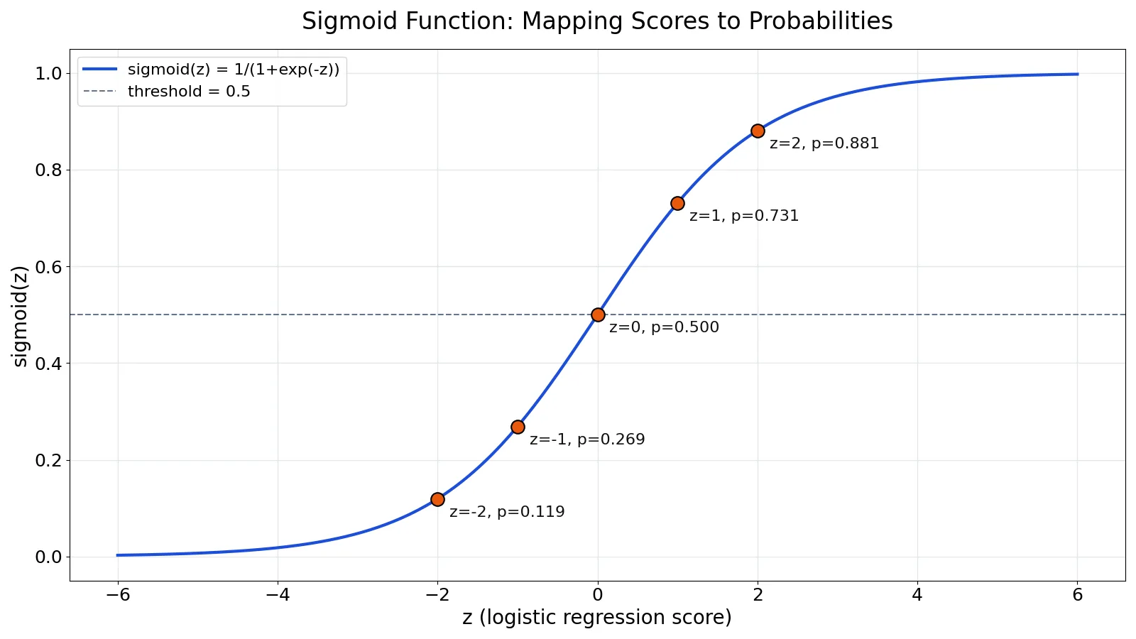
The sigmoid function is a mathematical function that takes any real number and squeezes it into a value between 0 and 1. That output range is exactly what you need when you want to model a probability, which is why logistic regression relies on it. This article covers the formula, how the curve behaves, and a worked example you can reproduce in Python or Excel.

Quick Answer

The sigmoid function is $\sigma(z) = \dfrac{1}{1 + e^{-z}}$, where $e$ is Euler's number (about 2.71828) [1].
Its output always falls between 0 and 1, no matter how large or small the input is [1].
At $z = 0$ the output is exactly 0.5, the midpoint of the curve.
Large positive inputs push the output toward 1, large negative inputs push it toward 0 [1].
Logistic regression passes a linear score $z$ through the sigmoid function to produce a probability [1].

What the Sigmoid Function Means

In plain terms, the sigmoid function is a smooth S-shaped curve that converts an unbounded number into a bounded one. Feed it a score of 500 and you get something very close to 1. Feed it -500 and you get something very close to 0. Feed it 0 and you get 0.5.

The precise definition: the sigmoid function, also called the standard logistic function, is defined for every real number $z$ as

$$\sigma(z) = \frac{1}{1 + e^{-z}}$$

Its domain is all real numbers and its range is the open interval $(0, 1)$. The function is continuous, monotonically increasing, and differentiable everywhere. Because it is monotonic, a larger input always produces a larger output, which keeps the ranking of scores intact after the transformation.

The curve is sometimes described as two exponential behaviors joined together. Early on, growth looks exponential, then a limiting factor flattens it toward a ceiling [2]. That shape shows up in population growth, adoption curves, and neural network activations, not only in classification [3][2].

How It Works

The formula has one input and one parameter-free shape:

$$\sigma(z) = \frac{1}{1 + e^{-z}}$$

$\sigma(z)$ is the output, a value strictly between 0 and 1.
$z$ is the input, often called the logit or log-odds. It can be any real number.
$e$ is Euler's number, the base of the natural logarithm, approximately 2.71828.
$e^{-z}$ is the exponential of the negated input. When $z$ is large and positive, $e^{-z}$ becomes tiny, so the denominator approaches 1 and the output approaches 1. When $z$ is large and negative, $e^{-z}$ becomes huge, so the output approaches 0.

In logistic regression, $z$ is not a raw feature. It is a linear combination of features and weights:

$$z = b + w_1x_1 + w_2x_2 + \ldots + w_Nx_N$$

Here $b$ is the bias, each $w_i$ is a weight, and each $x_i$ is a feature value. The model computes $z$, then passes it to the sigmoid function to get a probability [1]. The value $z$ is called the log-odds because it equals the natural logarithm of the ratio of the two outcome probabilities, $y$ and $1 - y$ [1].

The inverse relationship matters too. If you know a probability $p$, the log-odds are $\ln\left(\frac{p}{1-p}\right)$. The sigmoid function and the logit function undo each other.

Worked Example

The dataset below holds five students, each with a logistic regression score $z$ and a pass/fail outcome.

Student	z_score	passed
S1	-2	0
S2	-1	0
S3	0	1
S4	1	1
S5	2	1

Applying the formula $\sigma(z) = 1 / (1 + \exp(-z))$ to each score gives the following probabilities.

Student	z_score	Calculation	Probability
S1	-2	$1 / (1 + 7.3891)$	0.1192
S2	-1	$1 / (1 + 2.7183)$	0.2689
S3	0	$1 / (1 + 1.0000)$	0.5000
S4	1	$1 / (1 + 0.3679)$	0.7311
S5	2	$1 / (1 + 0.1353)$	0.8808

Notice the symmetry. The probability at $z = -2$ is 0.1192 and at $z = 2$ is 0.8808, and those two values sum to 1.0000. The same holds for $z = -1$ and $z = 1$, which give 0.2689 and 0.7311. This is a general property: $\sigma(-z) = 1 - \sigma(z)$.

Here is the same calculation in Python.

import math
def sigmoid(z):
    return 1 / (1 + math.exp(-z))
print(round(sigmoid(-2), 4))  # 0.1192

Output:

0.1192

In Excel, with the $z$ value in cell B2, the formula is =1/(1+EXP(-B2)), which returns 0.1192 for $z = -2$. If you need to round those outputs for a report, the Excel ROUND function handles that cleanly.

How to Interpret It

Read the output as a probability. A value of 0.8808 means the model estimates an 88.08% chance of the positive class. A value of 0.1192 means roughly a 12% chance [1].

The 0.5 point is the natural decision boundary. Scores above 0 push the probability above 0.5, scores below 0 push it below 0.5. At exactly $z = 0$ the model is indifferent.

The steepness near zero tells you how sensitive the model is. Around $z = 0$ a one-unit change in $z$ moves the probability by roughly 0.23, as you can see between S3 and S4. Far out in the tails, the same one-unit change barely moves the output at all. That saturation is why extreme scores produce probabilities that hug 0 or 1 without ever reaching them.

Because the output is a probability, it connects directly to other probability tools. If you treat each prediction as a single yes/no trial, the Bernoulli distribution is the underlying model, and the sigmoid output is its parameter.

When to Use It (and when not to)

Use the sigmoid function when you need a bounded output that behaves like a probability. Binary logistic regression is the classic case [1]. It also works as an activation function in neural networks, where it transforms a neuron's linear combination into a value between 0 and 1 [3].

Use it when you want a smooth, differentiable curve. Gradient-based training needs a derivative, and the sigmoid function has a convenient one: $\sigma'(z) = \sigma(z)(1 - \sigma(z))$.

Avoid it when your target is not binary. Multiclass problems need a softmax over several outputs, not a single sigmoid. Avoid it as a hidden-layer activation in deep networks, where it is prone to slow training because the gradient shrinks toward zero in the saturated regions [3]. ReLU often performs better there for that reason [3].

Avoid it when you need outputs outside $(0, 1)$. If your target can be negative or exceed 1, the sigmoid function is the wrong shape. A Gaussian function or a linear output fits better.

Sigmoid Function vs Logit Function

These two are inverses of each other, which is the most common source of confusion.

Property	Sigmoid function	Logit function
Input	Any real number $z$	A probability $p$ in $(0, 1)$
Output	A probability in $(0, 1)$	A real number
Formula	$\sigma(z) = \frac{1}{1 + e^{-z}}$	$\text{logit}(p) = \ln\left(\frac{p}{1-p}\right)$
Direction	Log-odds to probability	Probability to log-odds
Use in modeling	Final step of logistic regression	Interpreting coefficients as odds

If a coefficient in a logistic regression is 0.7, that is a change in log-odds. Exponentiating it gives the odds ratio. The sigmoid function is what turns the resulting log-odds back into a probability for a prediction [1].

Common Mistakes

Treating the sigmoid output as a class label. The output is a probability, not a decision. You still need a threshold to convert it into True or False [1]. Pick the threshold based on the cost of each error type.
Assuming the output can equal 0 or 1. It cannot. The curve approaches those values asymptotically but never reaches them, so a probability of exactly 0 or 1 only appears after rounding.
Confusing the sigmoid function with the logit function. They are inverses. Applying the wrong one sends your numbers in the wrong direction.
Using a sigmoid for multiclass targets. A single sigmoid gives one probability. For three or more mutually exclusive classes you need a softmax, which produces probabilities that sum to 1.
Ignoring saturation in the tails. A $z$ of 10 and a $z$ of 50 produce nearly identical probabilities. If your model relies on distinguishing extreme scores, the sigmoid function erases that difference.
Forgetting that $z$ is a linear combination. The sigmoid only shapes the output. All the feature engineering and weight fitting happens before it, in $z$.

Limitations

The sigmoid function cannot fix a poorly specified linear model. If $z$ does not separate the classes well, the sigmoid will faithfully compress a bad score into a confident-looking probability. The curve is also symmetric around 0.5, which assumes the two classes are treated symmetrically in the score space. When one class is rare, the raw output can look reasonable while the thresholded predictions are poor.

The saturation regions are a practical problem. Gradients become very small when $z$ is far from zero, which slows learning in neural networks and makes the model insensitive to changes in extreme inputs [3]. The function also gives no measure of uncertainty about its own output. A probability of 0.9 from a well-calibrated model and a probability of 0.9 from an overfit model look identical on the curve.

Frequently Asked Questions

What is the sigmoid function in simple terms?

It is a formula that takes any number and returns a value between 0 and 1. Very negative inputs give outputs near 0, very positive inputs give outputs near 1, and an input of 0 gives exactly 0.5. That range makes it useful for turning scores into probabilities.

Why does logistic regression use the sigmoid function?

Logistic regression needs an output that can be read as a probability, and the sigmoid function always returns a value between 0 and 1 [1]. It is also smooth and differentiable, so the model can be trained with gradient-based methods. The input to the sigmoid is the linear combination of features and weights [1].

What is the difference between the sigmoid function and the logistic function?

The standard logistic function is the specific sigmoid function $\sigma(z) = 1/(1+e^{-z})$ [1]. "Sigmoid" describes the S shape, and several functions share that shape. In machine learning the two terms are usually used interchangeably for this formula.

What is the sigmoid function at z = 0?

It equals 0.5. Substituting $z = 0$ gives $1/(1+e^{0}) = 1/(1+1) = 0.5$. This is the midpoint of the curve and the natural decision boundary in logistic regression.

Can the sigmoid function output exactly 0 or 1?

No. The output approaches 0 as $z$ goes to negative infinity and approaches 1 as $z$ goes to positive infinity, but it never equals either value for any finite input [1]. Any 0 or 1 you see in practice comes from rounding or from applying a threshold.

Is the sigmoid function still used in neural networks?

Yes, but mainly in the output layer for binary classification. In hidden layers, ReLU is often preferred because it is less susceptible to the vanishing gradient problem during training [3]. The sigmoid function remains a standard choice when you need a bounded probability as the final output.