Gamma Distribution Formula: PDF, Mean and Examples

By Dr. Zubair Khalid, DVM, MS, PhD · 2026-10-03

The gamma pdf is the probability density function of the gamma distribution, written $f(x) = \dfrac{x^{k-1} e^{-x/\theta}}{\theta^k \Gamma(k)}$ for $x \ge 0$. It has two parameters: a shape parameter $k$ (also written $\alpha$ or $a$) and a scale parameter $\theta$ (also written $\beta$). The gamma distribution models waiting times, lifetimes, and any positive quantity built from several exponential events added together.

Quick Answer

The gamma pdf is $f(x) = \dfrac{x^{k-1} e^{-x/\theta}}{\theta^k \Gamma(k)}$ for $x \ge 0$, with shape $k > 0$ and scale $\theta > 0$ [1].
The mean is $\mu = k\theta$ and the variance is $\sigma^2 = k\theta^2$ [2].
$\Gamma(k)$ is the gamma function, which equals $(k-1)!$ when $k$ is a positive integer [3].
When $k = 1$ the gamma reduces to the exponential distribution, and when $k$ is an integer it is also called the Erlang distribution [1].
Probabilities come from the cumulative distribution function $F(x) = \Gamma_x(k) / \Gamma(k)$, where $\Gamma_x(k)$ is the lower incomplete gamma function evaluated at $x/\theta$ [3].

The Formula

The gamma probability density function in the shape-scale parameterization is:

$$f(x) = \frac{x^{k-1} e^{-x/\theta}}{\theta^k \Gamma(k)}, \qquad x \ge 0,\ k > 0,\ \theta > 0$$

Each symbol has a specific job:

Symbol	Name	Meaning
$x$	Value	The point where you evaluate the density, such as a time or a rate
$k$	Shape parameter	Controls the shape. Also written $\alpha$ or $a$ [2]
$\theta$	Scale parameter	Stretches the distribution along the x-axis. Also written $\beta$ [2]
$\Gamma(k)$	Gamma function	Normalizing constant, $\Gamma(k) = \int_0^\infty t^{k-1} e^{-t} dt$ [3]
$e$	Euler's number	Base of the natural logarithm, about 2.71828

A second parameterization is common in the literature. It uses a rate parameter $b = 1/\theta$ and writes the density as $f(t) = \dfrac{b^a}{\Gamma(a)} t^{a-1} e^{-bt}$ [2]. The two forms describe the same distribution, so check which one a source is using before you plug in numbers.

The cumulative distribution function is:

$$F(x) = \frac{\Gamma_x(k)}{\Gamma(k)}$$

where $\Gamma_x(k) = \int_0^{x/\theta} t^{k-1} e^{-t} dt$ is the lower incomplete gamma function evaluated at $x/\theta$ [3]. There is no simple closed form for the CDF, so you evaluate it with software or statistical tables.

How to Calculate It Step by Step

Identify the shape $k$ and scale $\theta$ from your problem or your fitted model.
Check that $x \ge 0$. The gamma pdf is zero for negative values.
Compute the numerator $x^{k-1} e^{-x/\theta}$.
Compute the denominator $\theta^k \Gamma(k)$.
Divide the numerator by the denominator to get $f(x)$.
For a probability, use the CDF instead: $P(X \le x) = F(x)$, or subtract for a right-tail probability, $P(X > x) = 1 - F(x)$.

Step 6 matters because the pdf value itself is a density, not a probability. If you want the chance that a value falls in an interval, integrate the pdf over that interval, which is the same as subtracting two CDF values. The probability density function guide covers why densities can exceed 1 while probabilities cannot.

Worked Example

The dataset is lab instrument response times in seconds for 10 trials.

Trial	Response time (s)
1	0.8
2	1.4
3	2.1
4	2.7
5	3.3
6	4.0
7	4.6
8	5.2
9	6.1
10	7.5

Suppose the response times follow a gamma distribution with shape $k = 2.0$ and scale $\theta = 1.5$. Here is the full calculation.

Parameters. Shape $k = 2.0$, scale $\theta = 1.5$.

Mean. $\mu = k\theta = 2.0 \times 1.5 = 3.0000$.

Variance. $\sigma^2 = k\theta^2 = 2.0 \times 1.5^2 = 4.5000$.

Standard deviation. $\sigma = \sqrt{4.5000} = 2.1213$.

PDF numerator at $x = 3.0$. $x^{k-1} e^{-x/\theta} = 3.0^{1.0} \times e^{-3.0/1.5} = 3.0000 \times 0.1353 = 0.4060$.

PDF denominator. $\theta^k \Gamma(k) = 1.5^{2.0} \times \Gamma(2.0) = 2.2500 \times 1.0000 = 2.2500$.

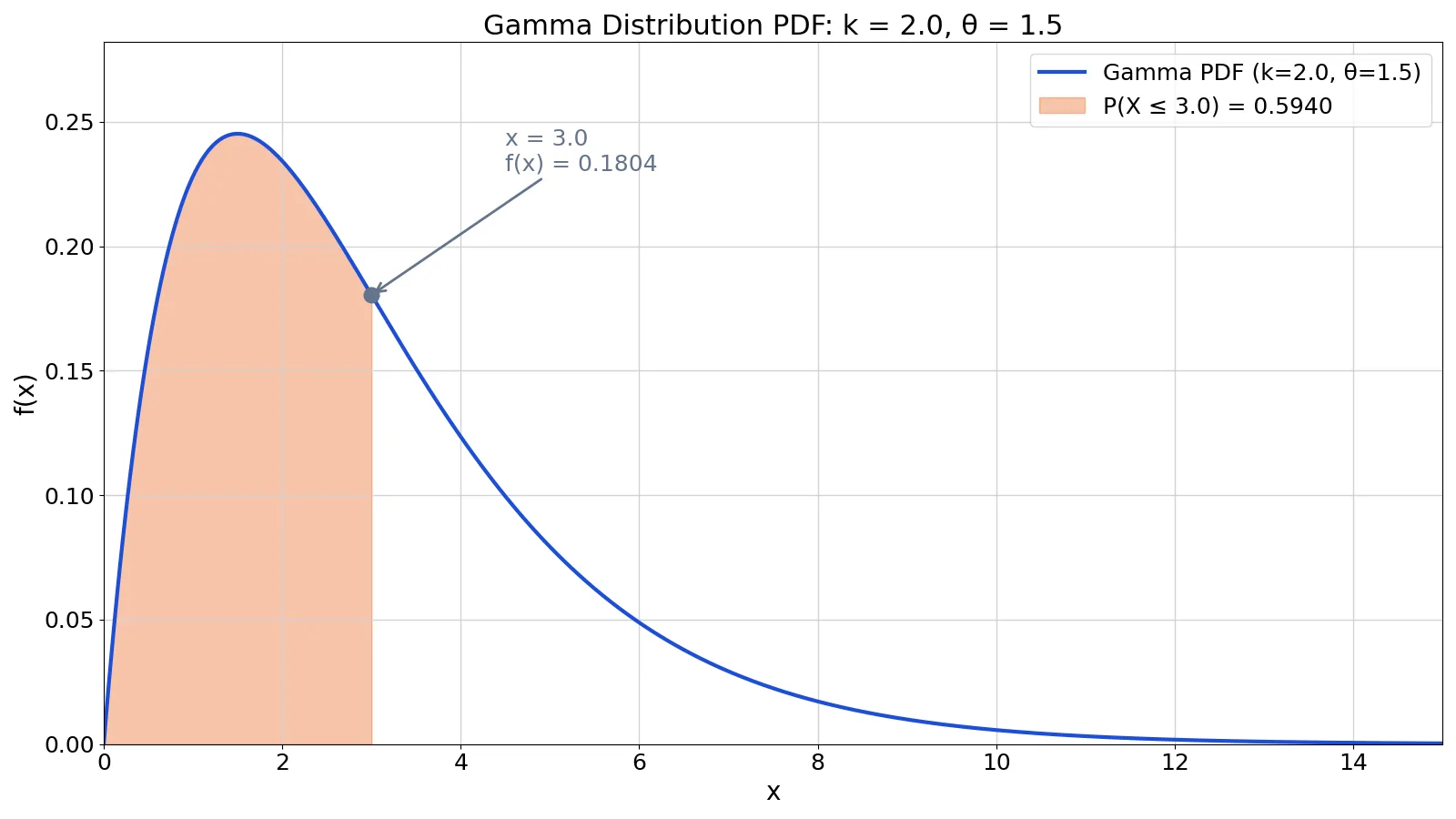
PDF at $x = 3$. $f(3.0) = 0.4060 / 2.2500 = 0.1804$.

CDF. $P(X \le 3.0) = 0.5940$.

So the density at the mean is 0.1804, and about 59.4% of response times are expected to fall at or below 3.0 seconds.

How to Interpret the Result

The value $f(3.0) = 0.1804$ is a density, not a probability. It tells you how concentrated the distribution is near 3.0 seconds. To turn it into a probability you need an interval. For a narrow interval of width $w$ around 3.0, the probability is roughly $0.1804 \times w$. For example, the chance of landing between 2.95 and 3.05 seconds is about $0.1804 \times 0.10 = 0.0180$.

The CDF value is directly interpretable. $P(X \le 3.0) = 0.5940$ means that under this model, roughly 59% of instrument response times are 3.0 seconds or less. The remaining 40.6% are longer. Because the mean is also 3.0, this example sits at the center of mass of the distribution, which is why the density is close to its peak region.

The shape parameter controls how skewed the curve is. With $k = 2.0$ the distribution is right-skewed, so long response times are possible even though most values cluster below the mean. As $k$ grows, the gamma looks more symmetric and approaches a normal shape. The normal PDF article shows what that limiting shape looks like.

Doing It in Software

Python's SciPy library computes the gamma pdf and CDF directly. The a argument is the shape and scale is the scale parameter [1].

from scipy.stats import gamma
k, theta, x = 2.0, 1.5, 3.0
pdf = gamma.pdf(x, a=k, scale=theta)
cdf = gamma.cdf(x, a=k, scale=theta)
print(f"pdf = {pdf:.4f}, cdf = {cdf:.4f}")  # pdf = 0.1804, cdf = 0.5940

Output:

pdf = 0.1804, cdf = 0.5940

In Excel, GAMMA.DIST(x, alpha, beta, cumulative) returns the gamma distribution. Set cumulative to TRUE for the CDF and FALSE for the pdf. Excel's beta argument is the scale parameter, matching the $\theta$ used here. GAMMA.INV(probability, alpha, beta) returns the inverse CDF, which is useful for finding percentiles.

In R, dgamma(x, shape = k, scale = theta) gives the pdf and pgamma(x, shape = k, scale = theta) gives the CDF. R's second positional argument is rate, so name scale explicitly as shown, or pass rate if your source uses the rate form.

Common Mistakes

Treating the pdf value as a probability. $f(3.0) = 0.1804$ is not an 18% chance. Fix: use the CDF for probabilities, or multiply the density by an interval width for an approximation.
Mixing up scale and rate. A scale of 1.5 means a rate of $1/1.5 = 0.6667$. Fix: check which parameterization your software expects. SciPy uses scale, R takes rate as its second positional argument unless you name scale, and Excel's beta is scale.
Forgetting that $x$ must be non-negative. The gamma pdf is zero for negative $x$. Fix: confirm your data are positive before fitting, and use a different distribution for data that can go below zero.
Assuming $k$ must be an integer. The shape parameter can be any positive real number. Fix: only use the factorial shortcut $\Gamma(k) = (k-1)!$ when $k$ is a positive integer [1].
Using the mean as a typical value without checking skew. For small $k$ the mean sits to the right of the peak. Fix: report the median or a percentile alongside the mean when the distribution is strongly skewed.
Confusing the gamma with the chi-square. A chi-square with $n$ degrees of freedom is a gamma with $a = n/2$ and $b = 0.5$ in the rate form, which is scale $\theta = 2$ [2]. Fix: convert parameters before reusing formulas.

Limitations

The gamma distribution only applies to positive continuous quantities. It cannot model data that take negative values, and it cannot model counts or proportions directly. If your data are counts, the Poisson distribution or the negative binomial distribution is the better fit.

Fitting a gamma to a small sample can be unstable. With 10 observations, the shape and scale estimates carry wide uncertainty, and a different sample could shift them noticeably. The gamma also assumes a single mode and a specific right-skewed shape. Data with two peaks or a sharp cutoff will not fit well, and forcing a gamma onto them produces misleading probabilities. For data bounded on both ends, the uniform distribution is a more honest starting point.

Frequently Asked Questions

What is the difference between the gamma pdf and the gamma CDF?

The pdf gives the density at a single point, which describes how concentrated the distribution is there. The CDF gives the probability that a value is less than or equal to a point. In the worked example, the pdf at 3.0 is 0.1804 and the CDF at 3.0 is 0.5940. Use the pdf for shape and the CDF for probabilities.

What does the shape parameter k control?

The shape parameter controls the form of the curve. When $k = 1$ the gamma becomes the exponential distribution, which peaks at zero and decays. As $k$ increases, the peak moves right and the curve becomes more symmetric. The scale parameter $\theta$ stretches the curve horizontally without changing its basic shape [1].

How do I find the mean and variance of a gamma distribution?

The mean is $k\theta$ and the variance is $k\theta^2$ [2]. With $k = 2.0$ and $\theta = 1.5$, the mean is 3.0000 and the variance is 4.5000, giving a standard deviation of 2.1213. These formulas hold for any positive values of $k$ and $\theta$.

Can the gamma pdf value be greater than 1?

Yes. A density is not a probability, so it has no upper bound of 1. When the scale is small, the distribution is tightly concentrated and the density can be large. Only the area under the curve must equal 1. This is the same property that applies to any continuous density, including the Student's t-distribution.

When should I use the gamma distribution instead of the normal distribution?

Use the gamma when your data are positive and right-skewed, such as waiting times, lifetimes, or rainfall amounts. Use the normal distribution when your data are roughly symmetric and can take negative values. For large shape parameters the gamma approaches a normal shape, so the choice matters most when $k$ is small.