Excel LEFT Function: Extract Text from the Left
By Dr. Zubair Khalid, DVM, MS, PhD ·
The Excel LEFT function returns the first character or characters in a text string, based on the number of characters you specify [1]. It is the standard way to pull a fixed-length prefix out of a cell, such as an area code, a product category or an ID segment. This article covers the syntax, a worked example, the errors you will hit and how to fix them.
Quick Answer
LEFT(text, num_chars)returns the firstnum_charscharacters oftext, counting from the left [1].textis required andnum_charsis optional. If you omitnum_chars, Excel assumes 1 [1].num_charsmust be greater than or equal to zero [1].- If
num_charsis larger than the length of the text, LEFT returns the whole string instead of an error [1]. - LEFT counts characters, so spaces, hyphens and digits all count toward the total.
Syntax
| Argument | Required? | Meaning |
|---|---|---|
text | Required | The text string that contains the characters you want to extract [1] |
num_chars | Optional | The number of characters you want LEFT to extract. Must be greater than or equal to zero. If omitted, it is assumed to be 1 [1] |
The formula pattern is:
$$=\text{LEFT}(\text{text},\ \text{num\_chars})$$
How It Works
LEFT walks the string from position 1 and stops after the number of characters you asked for. Position 1 is the first character on the left, so =LEFT("AB-1042",2) returns AB. Nothing about the rest of the string changes. LEFT does not trim spaces, does not convert numbers to text and does not look for a delimiter.
Two behaviors matter in practice. First, num_chars is optional, so =LEFT(A2) returns a single character [1]. Second, if num_chars exceeds the string length, LEFT returns all of the text rather than padding or erroring [1]. That makes LEFT safe to over-ask, which is useful when field lengths vary.
LEFT returns text, even when the extracted characters are digits. If you need the result as a number, wrap it in VALUE or multiply by 1. If you need to pull characters from the end of a string instead, the Excel RIGHT function is the mirror image of LEFT.
Worked Example
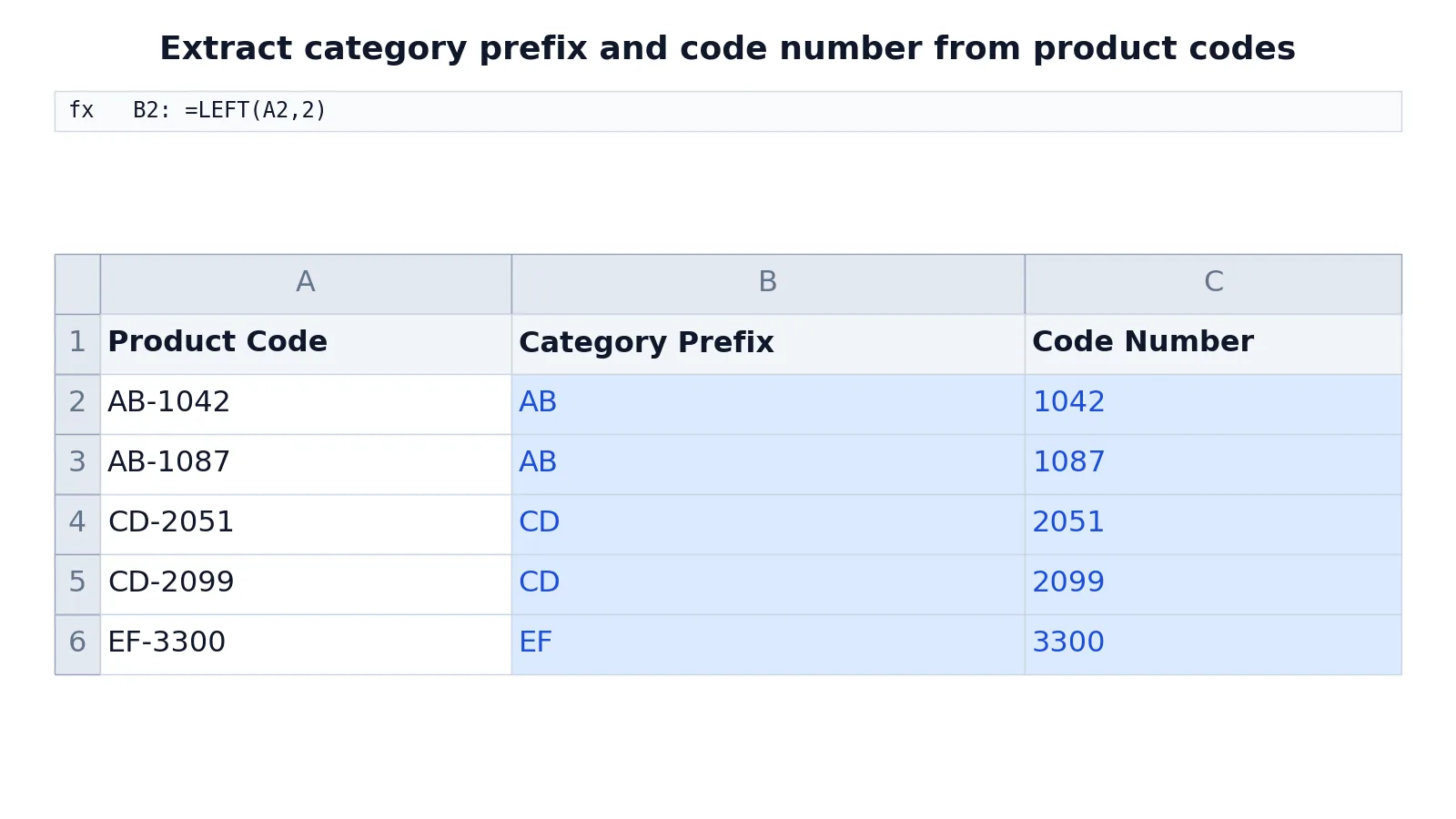
The table below holds product codes in column A. Column B extracts the two-letter category prefix with LEFT, and column C uses FIND to locate the hyphen so MID can return the numeric code.
| A | B | C | |
|---|---|---|---|
| 1 | Product Code | Category Prefix | Code Number |
| 2 | AB-1042 | =LEFT(A2,2) -> displays AB | =MID(A2,FIND("-",A2)+1,10) -> displays 1042 |
| 3 | AB-1087 | =LEFT(A3,2) -> displays AB | =MID(A3,FIND("-",A3)+1,10) -> displays 1087 |
| 4 | CD-2051 | =LEFT(A4,2) -> displays CD | =MID(A4,FIND("-",A4)+1,10) -> displays 2051 |
| 5 | CD-2099 | =LEFT(A5,2) -> displays CD | =MID(A5,FIND("-",A5)+1,10) -> displays 2099 |
| 6 | EF-3300 | =LEFT(A6,2) -> displays EF | =MID(A6,FIND("-",A6)+1,10) -> displays 3300 |
In B2, LEFT takes the first two characters of AB-1042 and returns AB. Filled down, B3 and B4 return AB and CD, and B5 and B6 return CD and EF. The prefix is now a clean grouping key you can sort, filter or count.
Column C shows the companion technique. FIND("-",A2) returns the position of the hyphen, and adding 1 gives the start of the number. MID then returns up to 10 characters from that position, which is more than enough for a four-digit code. The Excel FIND function is case-sensitive, so it is a good fit when your delimiter is a fixed symbol like a hyphen.
More Examples
Fixed-length ID segments. If every employee ID is formatted as EMP-00417, =LEFT(A2,3) returns EMP for every row. This is the simplest use of the function and the one you will reach for most often.
Area codes from phone numbers. For a 10-digit number stored as text, =LEFT(A2,3) returns the area code. If the number is stored as a real number, LEFT converts it to text first, so leading zeros are already gone. Store phone numbers as text if the leading zero matters.
Year from a date string. For text like 2024-03-15, =LEFT(A2,4) returns 2024. If the value is a true Excel date rather than text, use YEAR instead, because LEFT would read the underlying serial number.
Combining LEFT with other text functions. =LEFT(A2,LEN(A2)-3) drops the last three characters of any string, whatever its length. The Excel TEXT function can then format the result, and the Excel SUBTOTAL function can aggregate a column of extracted values once you convert them to numbers.
Nesting LEFT inside a lookup. Extracted prefixes work well as lookup keys. =MATCH(LEFT(A2,2),D:D,0) finds the prefix in a reference list, and the Excel MATCH function article covers the match types in detail. You can also feed LEFT results into Excel FILTER to return all rows sharing a prefix.
Errors and How to Fix Them
| Error | Cause | Fix |
|---|---|---|
#VALUE! | num_chars is negative or non-numeric | Use a number greater than or equal to zero [1] |
#NAME? | The function name is misspelled | Type LEFT exactly |
| Wrong characters returned | num_chars does not match the real field width | Count the characters in a sample value and adjust |
| Leading zeros missing | The source was stored as a number, not text | Format the source column as Text before entering the data |
| Result treated as text | LEFT always returns text | Wrap in VALUE or multiply by 1 when you need a number |
Common Mistakes
- Forgetting that
num_charsdefaults to 1.=LEFT(A2)returns one character, not the whole cell [1]. Always state the count explicitly unless you truly want a single character. - Counting characters by eye. A space counts as a character.
AB -1042with a space before the hyphen needs 3, not 2. Check withLENon a sample value. - Expecting LEFT to find a delimiter. LEFT has no idea where your hyphen or comma sits. Pair it with FIND or SEARCH when the field width varies.
- Using LEFT on numbers with leading zeros. Excel strips leading zeros from numeric entries, so
00123becomes123before LEFT ever sees it. Import or format the column as text. - Forgetting the result is text. A prefix like
1042extracted with LEFT will not sum or compare as a number until you convert it. - Hard-coding a length that varies by row. If some codes have two-letter prefixes and others have three, a fixed
num_charswill be wrong for part of the data. Use FIND to locate the delimiter instead.
Limitations
LEFT only works on a fixed number of characters from the start. It cannot search for a pattern, skip leading spaces or handle variable-length prefixes on its own. When the prefix length changes from row to row, you need FIND or SEARCH to locate the boundary and then feed that position into LEFT or MID. LEFT also returns text, so any downstream arithmetic needs an explicit conversion.
There is a second limit worth knowing. LEFT operates on the characters Excel stores in the cell, not on what the cell displays. If a number is formatted with a currency symbol or a date is formatted as 2024-03-15, LEFT reads the underlying value, not the formatted string. Convert with the TEXT function first if you need to extract from the displayed form.
Frequently Asked Questions
What is the difference between LEFT and LEFTB?
LEFT counts characters. LEFTB counts bytes and was designed for double-byte character sets. The LEFTB function is deprecated, and LEFT now supports Unicode surrogates through the Compatibility Version, Version 2 setting [1]. For everyday work, use LEFT.
Can LEFT return a number instead of text?
Not directly. LEFT always returns a text value, even when every extracted character is a digit. Wrap the result in VALUE, or multiply it by 1, to convert it. If the extracted string contains a thousands separator or a currency symbol, clean it first or the conversion will fail.
What happens if num_chars is bigger than the string?
LEFT returns the entire text string with no error [1]. This is convenient when field lengths vary, because you can set a generous count and let short values pass through unchanged. It also means a typo in num_chars can silently return more characters than you expected.
Is the Excel LEFT function case-sensitive?
No. LEFT does not compare characters, it only counts them, so case never affects the result. Case sensitivity becomes relevant when you pair LEFT with FIND, which is case-sensitive, or with SEARCH, which is not. Choose FIND when the delimiter is a fixed symbol and SEARCH when letter case varies.
How do I extract everything before a space?
Use =LEFT(A2,FIND(" ",A2)-1). FIND returns the position of the first space, and subtracting 1 excludes it. If a value might contain no space at all, wrap the formula in IFERROR so the #VALUE! error is replaced with a blank or the original text.
References
Further Reading
- Left, Mid, and Right functions - Power Platform | Microsoft Learn
- Broman KW, Woo KH (2018). Data Organization in Spreadsheets. The American Statistician
- Ziemann M, Eren Y, El-Osta A (2016). Gene name errors are widespread in the scientific literature. Genome Biology
- Microsoft Support: Excel help and learning
- McCullough B, Heiser DA (2008). On the accuracy of statistical procedures in Microsoft Excel 2007. Computational Statistics & Data Analysis