Excel FIND Function: Syntax, Examples and SEARCH Comparison
By Dr. Zubair Khalid, DVM, MS, PhD ·
If you need to know where a piece of text sits inside a longer string, find functions in Excel do exactly that. FIND returns the position of a substring as a number, counting from the first character of the text you search. It is case sensitive, so "AB" and "ab" are treated as different strings.
Quick Answer
- FIND returns the starting position of one text string inside another, as a number.
- The syntax is
FIND(find_text, within_text, [start_num]). find_textandwithin_textare required.start_numis optional and sets where the search begins.- FIND is case sensitive. SEARCH does the same job but ignores case [1].
- If the substring is not found, FIND returns the
#VALUE!error.
Syntax
| Argument | Required? | Meaning |
|---|---|---|
find_text | Required | The text you want to locate. |
within_text | Required | The text you search inside. |
start_num | Optional | The character position in within_text where the search starts. |
The function returns the position of the first character of find_text, measured from the first character of within_text [1].
How It Works
FIND scans within_text from left to right and stops at the first match. The value it returns is a position, not the text itself. If you search for "-" in AB-1042-XZ, the hyphen sits at position 3, so FIND returns 3.
The start_num argument changes where the scan begins. Setting start_num to 4 skips the first three characters, so the search ignores the hyphen at position 3 and finds the next one. This is the standard way to locate a second occurrence of the same character.
Positions are always counted from the first character of within_text, even when start_num is greater than 1. If you start at position 4 and the match is the eighth character of the string, FIND returns 8, not 5.
Case matters. FIND("a","Apple") fails because the capital A does not match the lowercase a. FIND("A","Apple") returns 1. If you need a case insensitive search, use SEARCH instead [1].
FIND does not support wildcard characters. The question mark and asterisk are treated as literal characters by FIND, while SEARCH treats them as wildcards. That difference matters when your text contains * or ?.
Worked Example
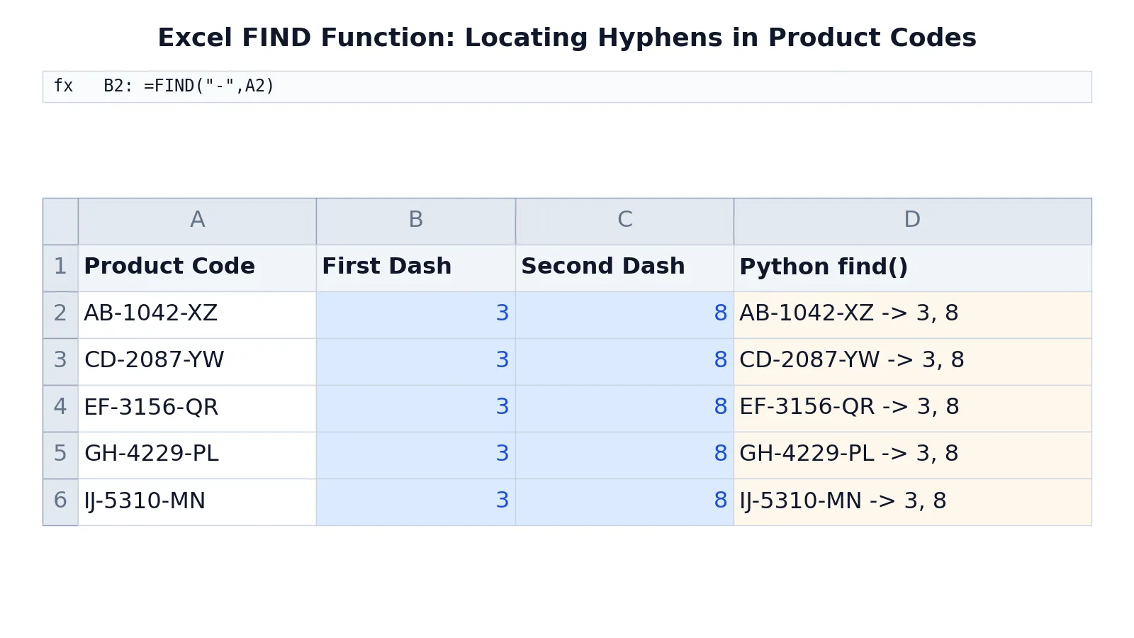
The table below uses a small product code list. Column A holds codes in the form AB-1042-XZ, and columns B and C pull out the positions of the two hyphens.
| A | B | C | D | |
|---|---|---|---|---|
| 1 | Product Code | First Dash | Second Dash | Python find() |
| 2 | AB-1042-XZ | =FIND("-",A2) -> displays 3 | =FIND("-",A2,4) -> displays 8 | =A2&" -> "&B2&", "&C2 -> displays AB-1042-XZ -> 3, 8 |
| 3 | CD-2087-YW | =FIND("-",A3) -> displays 3 | =FIND("-",A3,4) -> displays 8 | =A3&" -> "&B3&", "&C3 -> displays CD-2087-YW -> 3, 8 |
| 4 | EF-3156-QR | =FIND("-",A4) -> displays 3 | =FIND("-",A4,4) -> displays 8 | =A4&" -> "&B4&", "&C4 -> displays EF-3156-QR -> 3, 8 |
| 5 | GH-4229-PL | =FIND("-",A5) -> displays 3 | =FIND("-",A5,4) -> displays 8 | =A5&" -> "&B5&", "&C5 -> displays GH-4229-PL -> 3, 8 |
| 6 | IJ-5310-MN | =FIND("-",A6) -> displays 3 | =FIND("-",A6,4) -> displays 8 | =A6&" -> "&B6&", "&C6 -> displays IJ-5310-MN -> 3, 8 |
Cell B2 finds the first hyphen and returns 3. Cell C2 starts searching at position 4 and finds the second hyphen, which returns 8. Every code in the list follows the same two-letter, four-digit, two-letter pattern, so the results repeat down the column.
Once you have those positions, you can feed them into other text functions. The Excel RIGHT function can pull the trailing letters, and the Excel TEXT function can reformat the numeric part. The Excel INDEX function and Excel MATCH function pair well with FIND when you need to look up a parsed value.
More Examples
Find a space in a full name. =FIND(" ","Jane Doe") returns 5, because the space is the fifth character. You can then use that number with LEFT or MID to split the name.
Find a character after a fixed point. =FIND("@",A2,5) skips the first four characters before looking for the at sign. This helps when a string starts with a prefix you want to ignore.
Find a substring, not a single character. =FIND("base","database") returns 5, because "base" begins at the fifth character of "database" [1]. The same logic works for any multi-character search term.
Combine FIND with IFERROR. =IFERROR(FIND("-",A2),"none") returns the position when the hyphen exists and the text "none" when it does not. This keeps your sheet clean instead of showing an error.
Find the position of a number inside text. =FIND("1042","AB-1042-XZ") returns 4. FIND does not care whether the characters are letters or digits, only whether they match.
If you are new to text functions, the Excel functions overview explains how the categories fit together. For counting rather than locating, the COUNT function in Excel covers the numeric side.
Errors and How to Fix Them
#VALUE! when the text is not found. FIND returns #VALUE! if find_text does not appear in within_text. Wrap the formula in IFERROR or check your spelling.
#VALUE! when start_num is not a number. If start_num is text or a blank cell, FIND fails. Make sure the argument is a positive whole number.
#VALUE! when start_num is zero or negative. The starting position must be at least 1. A value of 0 or below triggers the error.
#VALUE! when start_num is larger than the string. If you start searching past the end of within_text, FIND cannot find anything and returns the error.
Unexpected results from case. FIND("x","Xylophone") fails because the lowercase x does not match the capital X. Switch to SEARCH if case should not matter [1].
Common Mistakes
- Assuming FIND ignores case. It does not. Use SEARCH when you want a case insensitive match [1].
- Forgetting that start_num counts from the start of the string. The returned position is always relative to the first character, not to
start_num. - Using FIND to test whether text exists. FIND returns a number or an error, so wrap it in ISNUMBER or IFERROR if you only need a yes or no answer.
- Expecting wildcards to work. FIND treats
*and?as ordinary characters. SEARCH treats them as wildcards [1]. - Hardcoding positions instead of calculating them. Positions shift when the source text changes, so let FIND do the counting.
- Ignoring the error instead of handling it. A stray
#VALUE!breaks downstream formulas that reference the cell.
Limitations
FIND only tells you where a substring starts. It cannot return the text around it, count how many times a substring appears, or search from right to left. To extract or replace text you have to pair it with functions like LEFT, MID, RIGHT or REPLACE [1].
FIND is also case sensitive and does not support wildcards, which makes it the wrong tool for fuzzy matching. If your data has inconsistent capitalization or you need pattern matching, SEARCH is the better choice [1]. Neither function handles multiple matches in one call, so finding the third or fourth occurrence means nesting FIND with a calculated start_num.
Frequently Asked Questions
What is the difference between FIND and SEARCH in Excel?
FIND is case sensitive and treats wildcard characters as literal text. SEARCH is not case sensitive and supports the ? and * wildcards [1]. Both return the starting position of the substring, and both accept the same three arguments. Choose FIND when case matters and SEARCH when it does not.
Why does FIND return #VALUE!?
The most common cause is that find_text does not exist in within_text. Other causes include a start_num that is zero, negative, non-numeric, or larger than the length of the string. Check each argument in turn to isolate the problem.
Is FIND case sensitive?
Yes. FIND("a","Apple") returns #VALUE! because the lowercase a does not match the capital A. FIND("A","Apple") returns 1. If you need a case insensitive search, use SEARCH instead [1].
How do I find the second occurrence of a character?
Use start_num to skip past the first match. If the first hyphen is at position 3, =FIND("-",A2,4) starts searching at position 4 and returns the position of the next hyphen. In the worked example above, that value is 8.
Can FIND work with numbers?
Yes. =FIND("1042","AB-1042-XZ") returns 4. If a cell holds a true number rather than text, FIND converts it to text automatically, so =FIND("4",1042) returns 2. Note that FIND scans the underlying value, not the formatted display.
Does FIND work in older versions of Excel?
FIND has been part of Excel for many versions and works in Excel 2016, 2019, 2021, 2024 and Microsoft 365 [1]. The syntax has not changed, so formulas built in older files continue to work in newer ones.
References
Further Reading
- Excel functions (by category) | Microsoft Support
- Broman KW, Woo KH (2018). Data Organization in Spreadsheets. The American Statistician
- Ziemann M, Eren Y, El-Osta A (2016). Gene name errors are widespread in the scientific literature. Genome Biology
- Microsoft Support: Excel help and learning
- McCullough B, Heiser DA (2008). On the accuracy of statistical procedures in Microsoft Excel 2007. Computational Statistics & Data Analysis