Skew to the Left vs Skewed Right: How to Tell the Difference

By Dr. Zubair Khalid, DVM, MS, PhD · 2026-10-03

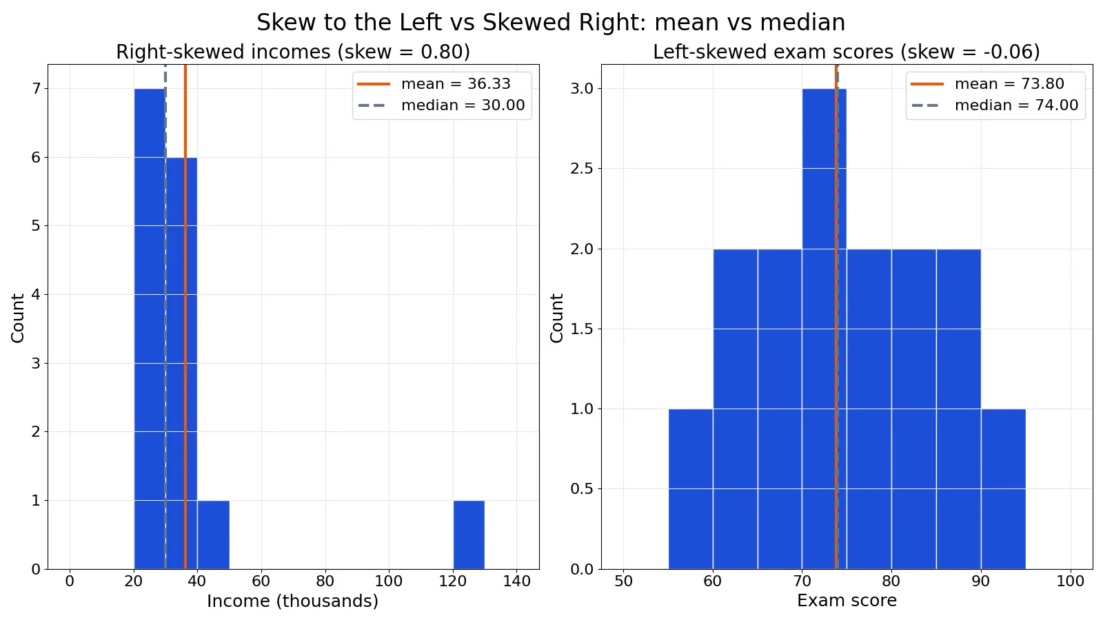
A distribution is skew to the left when its long tail stretches toward the smaller values, so the mean sits below the median. A distribution is skewed right when the long tail stretches toward the larger values, so the mean sits above the median. The direction of the tail, not the side where most data pile up, is what names the skew.

Quick Answer

Left skew (negative skew): the tail points left, the mean is less than the median, and the skewness value is negative [1].
Right skew (positive skew): the tail points right, the mean is greater than the median, and the skewness value is positive [1].
Symmetric data: the two halves of the histogram look like mirror images, the mean and median are close or the same, and skewness is near zero [2][3].
Fast check: subtract the median from the mean. A positive result points to right skew, a negative result points to left skew.
Best practice: read the histogram or box plot first, then confirm with the mean, median, and a skewness statistic [2].

Key Differences

Feature	Skew to the left	Skewed right
Long tail	Points to smaller values	Points to larger values
Mean vs. median	Mean < median	Mean > median
Skewness sign	Negative	Positive [1]
Typical cause	A ceiling effect (an upper bound), early failures [2]	A lower bound at zero, rare large values [2]
Effect on the mean	Pulled down by low outliers	Pulled up by high outliers

The comparison table is the fastest way to separate the two. If you only remember one row, remember the mean-versus-median row.

Left Skew Explained

Left skew is also called negative skew. The left tail is long relative to the right tail, which means a handful of unusually small values drag the mean downward [1]. The bulk of the data sits on the high side of the distribution.

Picture exam scores where most students score in the 70s and 80s but a few score very low. The histogram has a short right side and a long left tail. The mean drops below the median because those low scores pull it down.

The mean-median rule works because the mean responds to every value while the median only responds to position. Extreme values on the left move the mean left, and the median barely moves. That gap is the signal.

A box plot shows the same story. The left whisker is longer, and the median line sits closer to the right edge of the box. The article on reading skewness in box plots walks through that visual check step by step.

For a numeric measure, the Fisher-Pearson coefficient is the standard choice [1]. It is based on the third moment of the data:

$$ g_1 = \frac{\sum_{i=1}^{N}(Y_i - \bar{Y})^3 / N}{s^3} $$

Negative values indicate data that are skewed left, and positive values indicate data that are skewed right [1]. Many software packages apply a sample-size adjustment to this formula, and that adjustment approaches 1 as the sample grows [1]. SciPy's skew function computes the sample skewness and reports values near zero for normally distributed data [4].

Skewed Right Explained

Skewed right is also called positive skew. The right tail is long relative to the left tail, so a few unusually large values pull the mean upward [1]. Most of the data clusters on the low side.

Income is the classic example. Most people earn moderate amounts, and a small number earn far more. The histogram has a tall left cluster and a long right tail. The mean climbs above the median because the top earners pull it up.

Right skew is common when data have a lower bound of zero. Failure data must be non-negative, and many measurement processes generate only positive values, so time-to-occurrence and size measurements often come out right-skewed [2]. A reliability process with a long start-up period where failures are rare does the opposite: the few early failures form a long left tail, which is left skew [2].

The mean-median rule flips here. Mean greater than median means right skew. The right skewed distribution guide covers the same logic from the opposite direction.

Worked Example

This example uses 15 incomes (in thousands) and 15 exam scores from a small class survey.

Income	Score
22	55
24	60
25	62
26	65
27	68
28	70
29	72
30	74
31	76
32	78
33	80
35	82
38	85
45	88
120	92

Income dataset (n=15). The mean is $545/15 = 36.3333$. The median is the 8th sorted value, which is $30.0000$. The sample standard deviation is $23.8767$. The Pearson skew is:

$$3(36.3333 - 30.0000)/23.8767 = 0.7958$$

The mean is above the median, so the incomes are right-skewed. The single value of 120 pulls the mean up while the median stays at 30.

Score dataset (n=15). The mean is $1107/15 = 73.8000$. The median is the 8th sorted value, which is $74.0000$. The sample standard deviation is $10.6851$. The Pearson skew is:

$$3(73.8000 - 74.0000)/10.6851 = -0.0562$$

The mean is slightly below the median, so the scores lean left. The skew is small, which tells you the scores are close to symmetric.

Here is the code that produced those values:

import statistics as st
incomes = [22,24,25,26,27,28,29,30,31,32,33,35,38,45,120]
scores  = [55,60,62,65,68,70,72,74,76,78,80,82,85,88,92]
for name, x in [('income', incomes), ('score', scores)]:
    m = sum(x)/len(x); med = st.median(x); sd = st.stdev(x)
    print(f"{name:<6} {m:.4f} {med:.4f} {sd:.4f} {3*(m-med)/sd:.4f}")

Output:

income 36.3333 30.0000 23.8767 0.7958
score  73.8000 74.0000 10.6851 -0.0562

The quartiles tell the same story. Incomes have Q1 = 26.5 and Q3 = 34, so the upper half spreads wider. Scores have Q1 = 66.5 and Q3 = 81, a tighter and more even spread.

Which One Should You Use?

You do not choose the skew. The data has it, and your job is to report it correctly. What you choose is the summary statistic that best represents a typical value.

For skewed data, the median is usually the better measure of center because it resists the pull of the tail [2]. The mean is still useful, but it describes the balance point of the data, not the typical case.

If you need a formal test, SciPy's skewtest checks whether a skewness value is far enough from zero to be statistically meaningful [5]. For the sequence [1, 2, 3, 4, 5, 6, 7, 8000], the test returns a statistic of 3.5718 and a p-value of 0.0004, which flags clear right skew [5]. For [1, 2, 3, 4, 5, 6, 7, 8], the statistic is 1.0108 with a p-value of 0.3121, which does not flag skew [5].

If you want to model the data, skewed distributions often call for something other than the normal curve. Log or square root transformations are common for right-skewed data, and reliability studies often use the exponential, Weibull, or lognormal distributions instead of the normal [1].

Common Mistakes

Naming the skew after the tall side of the histogram. The name comes from the tail, not the peak. Fix: point at the long tail and name that direction.
Trusting the mean-median gap in tiny samples. With few values, one outlier can flip the sign. Fix: check the histogram and a skewness value together.
Treating a small skewness as proof of symmetry. A value like -0.0562 is close to zero and suggests near-symmetry, but it is not a formal test. Fix: run a skewness test when the decision matters [5].
Comparing skewness values across different sample sizes without care. Software adjustments change the value as N grows [1]. Fix: report which formula your tool uses.
Assuming skew means the data is bad. Skew is a property, not a defect. Fix: choose statistics and models that suit the shape.
Reading a box plot as if the median must sit in the middle of the box. It does not. Fix: judge skew from whisker lengths and the median's position inside the box.

Limitations

The mean-median rule is a heuristic, not a proof. It can point the wrong way when the distribution has more than one peak, when the sample is very small, or when the skew is mild. A mean-median gap of a fraction of a standard deviation tells you very little on its own.

Skewness values are also sensitive to outliers because they use cubed deviations. One extreme point can dominate the calculation. The histogram remains the most honest first look, and the numeric measures should confirm what you see there, not replace it.

Frequently Asked Questions

What does skew to the left mean in simple terms?

It means the long tail of the distribution points toward the smaller values. Most of the data sits on the high side, and a few low values stretch the left side out. The mean ends up below the median.

Is left skew the same as negative skew?

Yes. Left skew and negative skew describe the same shape. The skewness value is negative because the left tail is long relative to the right tail [1]. Right skew is the positive version of the same idea.

How do I tell left skew from right skew using the mean and median?

Subtract the median from the mean. A negative result means left skew, and a positive result means right skew. In the worked example, incomes gave $36.3333 - 30.0000 = 6.3333$, a positive gap and right skew. Scores gave $73.8000 - 74.0000 = -0.2000$, a negative gap and left skew.

Can a distribution be skewed left and right at the same time?

No. A single distribution has one tail that is longer, so it leans one way. If both tails look long, the shape may be symmetric with heavy tails on both sides, which is a kurtosis question, not a skew question [1].

What skewness value counts as close to zero?

There is no universal cutoff. For normally distributed data the skewness should be about zero, and symmetric data should have a skewness near zero [1][4]. Whether a given value is far enough from zero to matter depends on your sample size, so use a formal test like skewtest when the answer affects a decision [5].