What Is a Bayesian Model? Definition and Examples

By Dr. Zubair Khalid, DVM, MS, PhD · 2026-10-03

A Bayesian model is a statistical model in which unknown quantities are treated as random variables with probability distributions, and those distributions are updated when data arrive. You start with a prior distribution that encodes what you believe before seeing the data, then apply Bayes' theorem to combine that prior with the likelihood of the observed data. The result is a posterior distribution, which is your updated belief about the unknown quantity.

Quick Answer

A Bayesian model has three parts: a prior distribution, a likelihood for the data, and a posterior distribution produced by combining them.
The core formula is $P(\theta \mid D) \propto P(D \mid \theta) \times P(\theta)$, where $\theta$ is the unknown parameter and $D$ is the data [1].
The prior $P(\theta)$ states what you believe about $\theta$ before seeing data. The likelihood $P(D \mid \theta)$ states how probable the data are for each possible value of $\theta$.
The posterior $P(\theta \mid D)$ is the answer. It is a full probability distribution, so you can read a mean, a mode, and an interval directly from it.
Bayesian models extend naturally to comparing several models at once, since each model can carry its own prior probability and receive a posterior weight [1].

What a Bayesian Model Means

In plain terms, a Bayesian model is a way of learning from data while keeping track of what you already believed. You write down your starting belief as a probability distribution, you write down how the data would look under each possible value of the unknown quantity, and you let the data shift your belief.

The precise statistical definition is this. Let $\theta$ be the parameter or set of parameters you want to learn about, and let $D$ be the observed data. A Bayesian model specifies a prior distribution $p(\theta)$ and a likelihood $p(D \mid \theta)$. Inference then targets the posterior distribution

$$p(\theta \mid D) = \frac{p(D \mid \theta)\, p(\theta)}{p(D)}$$

where $p(D) = \int p(D \mid \theta)\, p(\theta)\, d\theta$ is the marginal likelihood, a normalizing constant that makes the posterior integrate to one. Because $p(D)$ does not depend on $\theta$, it is common to work with the proportional form $p(\theta \mid D) \propto p(D \mid \theta)\, p(\theta)$.

This is the same machinery as Bayes' theorem, applied to a parameter instead of an event. The parameter is a random variable with a distribution, and the distribution changes as evidence accumulates.

How It Works

The mechanism has four moving parts.

$\theta$ is the unknown quantity. It could be a coin's bias, a regression coefficient, or a failure rate.
$p(\theta)$ is the prior. It is a probability density over the possible values of $\theta$ before the data are seen.
$p(D \mid \theta)$ is the likelihood. It measures how well each candidate value of $\theta$ explains the observed data. This is the same object that maximum likelihood estimation maximizes.
$p(\theta \mid D)$ is the posterior. It combines the two and is the object you report.

The update is multiplicative. Values of $\theta$ that the prior favors and that the likelihood also favors get boosted. Values that one part favors but the other does not get pulled back. When the prior is flat or vague, the posterior is driven mostly by the likelihood. When data are scarce, the prior has more influence.

For a single model, the posterior is the whole answer. For a set of competing models $M_1, \dots, M_m$, you assign each a prior probability $P(M_i)$ and compute a weight $W_i = P(D \mid M_i) \times P(M_i)$. The posterior probability of each model is then $P(M_i \mid D) = W_i / \sum_{i=1}^{m} W_i$ [1]. Predictions average across all models using those weights, so no model is discarded outright [1].

When the prior and likelihood come from matching families, the posterior stays in the same family and the update reduces to simple arithmetic. This is called conjugacy. The beta-binomial pair used below is the standard example. When no conjugate form exists, you typically draw samples from the posterior with Markov chain Monte Carlo instead of solving the integral by hand.

Worked Example

The dataset is a sequence of 12 coin flips, with 10 heads and 2 tails. You want to estimate the coin's probability of heads, call it $\theta$.

flip_index	result
1	H
2	H
3	T
4	H
5	H
6	H
7	H
8	T
9	H
10	H
11	H
12	H

Step 1. Observed data. 10 heads out of 12 flips, so 2 tails.

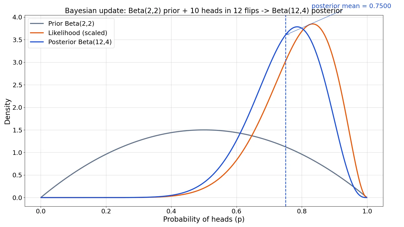
Step 2. Prior. You choose a Beta(2, 2) prior, which is symmetric and mildly favors values near 0.5. Its mean is $2/(2+2) = 0.5000$.

Step 3. Posterior parameters. The beta prior is conjugate to the binomial likelihood, so the update is just addition. The posterior is Beta with $a_1 = a_0 + \text{heads} = 2 + 10 = 12$ and $b_1 = b_0 + \text{tails} = 2 + 2 = 4$.

Step 4. Posterior mean. $a_1/(a_1+b_1) = 12/(12+4) = 0.7500$. The prior mean was 0.5000, so the data moved the estimate upward.

Step 5. Posterior mode. $(a_1-1)/(a_1+b_1-2) = 11/14 = 0.7857$. The mode sits above the mean because the posterior is slightly left-skewed.

Step 6. 95% credible interval. $[0.5191, 0.9221]$. This is the range that contains 95% of the posterior probability.

Here is the code that produces those numbers.

from scipy import stats
a0, b0 = 2, 2
heads, tails = 10, 2
a1, b1 = a0 + heads, b0 + tails
post_mean = a1 / (a1 + b1)
ci = stats.beta.ppf([0.025, 0.975], a1, b1)

Output:

posterior mean = 0.7500; 95% credible interval = [0.5191, 0.9221]

The figure shows the grey prior Beta(2, 2), the orange scaled likelihood, and the blue posterior Beta(12, 4), with a dashed line at the posterior mean of 0.7500. The posterior sits between the prior and the likelihood, closer to the likelihood because 12 flips carry more information than a Beta(2, 2) prior.

How to Interpret It

Read the posterior as a complete statement of uncertainty. The mean of 0.7500 is your point estimate. The mode of 0.7857 is the single most probable value. The 95% credible interval of $[0.5191, 0.9221]$ says that, given the prior and the data, there is a 0.95 posterior probability that $\theta$ lies in that range.

That last sentence is the key difference from a confidence interval. A credible interval is a direct probability statement about the parameter. A confidence interval is a statement about the procedure, not about the specific interval you computed. This is why Bayesian intervals are often easier to explain to a non-technical audience.

You can also read the posterior as a compromise. The prior mean was 0.5000, the data alone would suggest 10/12 = 0.8333, and the posterior mean landed at 0.7500. The prior pulled the estimate down, and the data pulled it up. Change the prior and the posterior changes with it, which is exactly the behavior you want when you have real prior information and exactly the behavior you must justify when you do not.

When to Use It (and when not to)

Use a Bayesian model when you have genuine prior information that should influence the estimate, such as earlier test results on the same system or a known physical bound on a parameter [2]. Use it when you want a probability distribution over parameters instead of a single point, or when you need to compare many models and average their predictions [1]. Use it when sample sizes are small and a well-chosen prior stabilizes the estimate. Use it when the model is hierarchical, since Bayesian methods handle grouped and nested structure naturally [3].

Avoid it when you have no defensible prior and no way to check sensitivity, because the answer will depend on a choice you cannot justify. Avoid it when a simple frequentist estimate is what your audience expects and the extra machinery adds nothing. Avoid it when the posterior cannot be computed in reasonable time and no approximation is acceptable. Also be careful with very large or very complex models, where sampling can be slow and convergence is hard to verify [4].

Bayesian Model vs Frequentist Model

Aspect	Bayesian model	Frequentist model
Parameter	Random variable with a distribution	Fixed unknown constant
Prior information	Encoded explicitly in a prior	Not used
Output	Full posterior distribution	Point estimate plus interval
Interval meaning	Probability the parameter is in the range	Long-run coverage of the procedure
Small samples	Prior helps stabilize estimates	Estimates can be unstable
Model comparison	Posterior weights across models [1]	Hypothesis tests or information criteria

The practical difference is where the probability lives. In a Bayesian model, probability describes your uncertainty about the parameter. In a frequentist model, probability describes the behavior of the estimator across repeated samples. Both are valid, and the right choice depends on the question and on what prior information you actually have.

Common Mistakes

Treating the prior as optional. Every Bayesian model has one, even if it is flat. If you do not state it, you cannot check how much it drives the result. Fix: always report the prior and run a sensitivity check with a different one.
Confusing the credible interval with a confidence interval. They answer different questions. Fix: describe the credible interval as a posterior probability statement and never as a coverage guarantee.
Using a vague prior on a scale where it is not vague. A flat prior on one parameter can be strongly informative on a transformed parameter. Fix: check the prior on the scale you actually care about.
Ignoring the normalizing constant. The posterior must integrate to one. Fix: when working in proportional form, confirm the result is a proper distribution before reporting it.
Reporting only the posterior mean. The mean hides skew and multimodality. Fix: report the mean, the mode, and an interval together.
Forgetting that the likelihood must match the data-generating process. A conjugate update is only valid if the likelihood is correct. Fix: check the model assumptions before trusting the arithmetic.

Limitations

A Bayesian model cannot create information that is not there. If the data are uninformative and the prior is strong, the posterior will mostly reflect the prior, and the result will look precise while being driven by an assumption. This is the most common way Bayesian results mislead.

The marginal likelihood $p(D)$ is often intractable, so real applications rely on sampling or approximation. Those methods can fail to converge, and the diagnostics that detect failure are not foolproof [4]. Bayesian nonparametric models push this further by replacing finite-dimensional priors with infinite-dimensional stochastic processes, which increases flexibility and also increases the computational burden [3]. Finally, the choice of prior is a modeling decision, not a neutral default, and it should be reported and defended like any other modeling choice.

Frequently Asked Questions

What is a Bayesian model in simple terms?

It is a model that starts with a probability distribution for what you believe, updates that distribution with observed data, and returns a new distribution as the answer. The update uses Bayes' theorem. You get a full picture of uncertainty instead of a single number.

What is the difference between a prior and a posterior?

The prior is your belief about the parameter before seeing the data. The posterior is your belief after combining the prior with the likelihood of the data. In the coin example, the prior mean was 0.5000 and the posterior mean was 0.7500.

Do I always need a prior distribution?

Yes. Every Bayesian model has one, even when it is chosen to be flat or weakly informative. The honest approach is to state the prior, explain why you chose it, and show that your conclusions do not hinge on it.

How do I choose a prior?

Use previous data, expert judgment, or a weakly informative default that rules out impossible values without pushing the estimate in a particular direction [2]. Then test sensitivity by refitting with a different prior and comparing the posteriors.

Can a Bayesian model be used for prediction?

Yes. You form a posterior predictive distribution by averaging the likelihood over the posterior. For multiple models, predictions are a weighted average across all models, with weights equal to the posterior model probabilities [1]. This is one of the main reasons Bayesian methods are used for forecasting and reliability work [2].