Maximum Likelihood Estimation: Definition and Example

By Dr. Zubair Khalid, DVM, MS, PhD · 2026-10-03

Maximum likelihood estimation is a method for estimating the parameters of a probability model from observed data. You pick the parameter values under which the data you actually saw would have been most likely to occur. The value that maximizes that probability is called the maximum likelihood estimate.

Quick Answer

Maximum likelihood estimation (MLE) asks one question: which parameter value makes the data I observed most probable? [1]
You write a likelihood function, which is the probability of the observed data expressed as a function of the unknown parameter. [2]
In practice you maximize the log-likelihood, since the logarithm turns products into sums and does not move the maximum. [1]
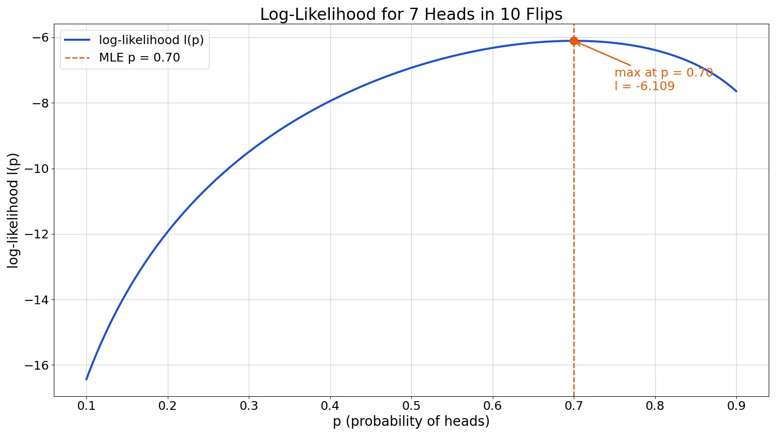
For 7 heads in 10 coin flips, the maximum likelihood estimate is $\hat{p} = 7/10 = 0.7000$, and the log-likelihood there is $-6.1086$.
MLE is a dominant method in statistical inference, but its best properties are large-sample properties. [1][3]

What Maximum Likelihood Estimation Means

In plain terms, maximum likelihood estimation is a way of asking which version of a model best explains the data you collected. You assume a probability distribution, then search over its unknown parameters for the setting that gives your observed sample the highest probability.

The precise definition: given independent observations $x_1, \dots, x_n$ from a distribution with density or probability mass function $f(x \mid \theta)$, the likelihood function is

$$L(\theta) = \prod_{i=1}^{n} f(x_i \mid \theta)$$

The maximum likelihood estimate is the point in the parameter space that maximizes $L(\theta)$. [1] Because products of many small probabilities underflow quickly, analysts almost always work with the log-likelihood instead:

$$\ell(\theta) = \sum_{i=1}^{n} \ln f(x_i \mid \theta)$$

This is the sample analogue of the expected log-likelihood. [1] The parameter value that maximizes $\ell(\theta)$ is the same one that maximizes $L(\theta)$, because the natural logarithm is strictly increasing.

How It Works

The mechanism has four steps.

Choose a model. Decide which distribution could have generated the data, such as a binomial for counts of successes or a normal for continuous measurements.
Write the likelihood. Multiply the probability of each observation together, treating the data as fixed and the parameter as the variable. [2]
Take the log. Convert the product into a sum, which is far easier to differentiate. See What Is Log-Likelihood? for the full treatment.
Maximize. Set the derivative of the log-likelihood with respect to the parameter to zero and solve. When a closed-form solution does not exist, numerical optimization finds the peak. [4]

Each symbol in the formulas above means the following. $x_i$ is the $i$-th observation. $\theta$ is the unknown parameter or vector of parameters. $f(x_i \mid \theta)$ is the probability of observation $x_i$ given $\theta$. $n$ is the sample size. $L(\theta)$ is the likelihood, and $\ell(\theta)$ is its natural logarithm.

The derivative condition for a single parameter is

$$\frac{d\ell}{d\theta} = 0$$

Solving that equation gives the estimate. For many standard models the solution is a simple function of the data, and for others it requires iterative software. [4][3]

Worked Example

The dataset is 10 coin flips with 7 heads, which we treat as independent draws from a Bernoulli distribution with unknown success probability $p$.

flip	outcome
1	H
2	H
3	H
4	H
5	H
6	H
7	H
8	T
9	T
10	T

Step 1: Data. We have $n = 10$ flips and $k = 7$ heads.

Step 2: Likelihood. Each head contributes a factor of $p$ and each tail a factor of $1-p$, so

$$L(p) = p^7 (1-p)^3$$

Step 3: Log-likelihood. Taking logs turns the product into a sum:

$$\ell(p) = 7\ln(p) + 3\ln(1-p)$$

Step 4: Derivative. Differentiate with respect to $p$ and set the result to zero:

$$\frac{d\ell}{dp} = \frac{7}{p} - \frac{3}{1-p} = 0$$

Step 5: Solve. Rearranging gives $7(1-p) = 3p$, so $p = 7/10 = 0.7000$. The maximum likelihood estimate is the observed proportion of heads.

Step 6: Check the peak. Evaluating the log-likelihood at three candidate values shows that 0.70 is the highest:

$p$	$\ell(p)$
0.5	-6.9315
0.7	-6.1086
0.9	-7.6453

The same answer comes out of numerical optimization:

from scipy.optimize import minimize_scalar
import numpy as np
n, k = 10, 7
neg_ll = lambda p: -(k*np.log(p) + (n-k)*np.log(1-p))
res = minimize_scalar(neg_ll, bounds=(0.01, 0.99), method='bounded')
print(round(res.x, 4))  # 0.7000

Output:

0.7

The log-likelihood curve rises to a single peak at $p = 0.70$ with $\ell = -6.109$, then falls away on both sides. That peak is the maximum likelihood estimate.

How to Interpret It

The estimate $\hat{p} = 0.70$ means that among the parameter values you considered, 0.70 makes the observed sequence of 7 heads and 3 tails most probable. It is not a claim that the coin is fair or unfair. It is the value your model and data jointly favor.

The log-likelihood values are negative because probabilities are below 1, and their logs are negative. What matters is the comparison, not the absolute size. The gap between $-6.1086$ at $p = 0.70$ and $-6.9315$ at $p = 0.50$ means the data are more plausible under 0.70 than under 0.50. The gap between $-6.1086$ and $-7.6453$ at $p = 0.90$ says the same about 0.90.

The estimate is a point estimate. It carries no built-in measure of uncertainty, so you usually pair it with a standard error or confidence interval. For a broader treatment of how estimates relate to populations, see Statistical Parameter: Definition, Types, and Estimation.

When to Use It (and when not to)

Use maximum likelihood estimation when you have a plausible probability model, independent observations, and a parameter you want to estimate. It applies to a wide range of situations, including censored data in reliability analysis, where some units have not yet failed. [2][3] It also extends to regression settings such as Generalized Linear Models, where the coefficients are estimated by maximizing a likelihood.

Avoid leaning on it when your sample is very small. Maximum likelihood estimates can be heavily biased in small samples, and the optimality properties may not apply. [3] It can also be sensitive to the choice of starting values in numerical optimization. [3]

Do not use it when you have strong prior information that should shape the answer. In that case a Bayesian approach, which combines a prior with the likelihood, is the natural alternative. See What Is a Bayesian Model? for how that works.

Maximum Likelihood Estimation vs Bayesian Estimation

Both approaches use the likelihood. They differ in what they do with it.

Aspect	Maximum likelihood estimation	Bayesian estimation
Input	Likelihood only	Likelihood plus a prior
Output	A single point estimate	A full posterior distribution
Prior information	Not used	Explicitly incorporated
Small samples	Can be biased [3]	Prior can stabilize estimates
Interpretation	Parameter value that makes the observed data most probable	Updated belief about the parameter

If you want one number and have little prior knowledge, maximum likelihood estimation is the direct route. If you want a distribution over plausible values, or you have real prior information, the Bayesian route fits better. The two are connected through Bayes' Theorem.

Common Mistakes

Maximizing the likelihood of the parameter instead of the data. The likelihood is a function of the parameter with the data held fixed. It is not the probability of the parameter. Fix: read $L(\theta)$ as "probability of the observed data, viewed as a function of $\theta$."
Forgetting to take the log. Multiplying many small probabilities produces numbers too small for most software to handle. Fix: work with the sum of logs, which peaks in the same place.
Reporting the estimate without uncertainty. A point estimate alone hides how precise it is. Fix: add a standard error or confidence interval.
Ignoring small-sample bias. MLE can be noticeably biased when $n$ is small. [3] Fix: check whether a bias-corrected estimator is available for your model.
Trusting a numerical optimizer blindly. Results can depend on starting values. [3] Fix: try several starting points and confirm the optimizer converged.
Assuming the model is correct. The estimate is only as good as the distribution you assumed. Fix: check model assumptions before interpreting the result, as covered in Understanding Model Assumptions in Statistical Analysis.

Limitations

Maximum likelihood estimation has no optimality guarantees for finite samples. Other estimators can concentrate more tightly around the true parameter value when the sample is small. [1] The attractive properties, including consistency, are limiting properties that describe behavior as the sample size grows toward infinity. [1]

The method is also computationally demanding in realistic settings. Except for a few cases where the formulas are simple, it is generally best to rely on high quality statistical software. [3] Multi-parameter problems often require setting partial derivatives of the log-likelihood to zero and solving a nonlinear system, which is complicated and only practical with appropriate software. [4] Finally, the estimate is conditional on the model. A wrong distribution or a violated independence assumption can produce a confidently wrong answer.

Frequently Asked Questions

What is the difference between a likelihood and a probability?

A probability describes how likely different data outcomes are for a fixed parameter value. A likelihood describes how plausible different parameter values are for a fixed set of observed data. The formula can look identical, but the roles are reversed. In maximum likelihood estimation you treat the data as fixed and vary the parameter.

Why do we maximize the log-likelihood instead of the likelihood?

The logarithm is a strictly increasing function, so it does not change where the maximum occurs. It converts a product of many terms into a sum, which is much easier to differentiate and far less prone to numerical underflow. This is why the log-likelihood is the standard working form. [1]

Is the maximum likelihood estimate always the sample proportion?

No. That result is specific to the binomial and Bernoulli models. For a normal distribution, the maximum likelihood estimate of the mean is the sample mean, but the estimate of the variance divides the sum of squared deviations by $n$ instead of $n-1$, which makes it a biased estimator of the population value. [5] Other models produce other formulas.

Can maximum likelihood estimation be used with censored data?

Yes. It applies to every form of censored or multicensored data, and it can estimate distribution and acceleration model parameters at the same time. [2][4] The likelihood is adjusted so that censored observations contribute the probability of surviving past their censoring time instead of a density value.

How do I know if my maximum likelihood estimate is reliable?

Check the sample size, the model assumptions, and the optimizer's convergence. Large samples support the consistency property, while small samples may carry bias. [1][3] Report a standard error or interval alongside the point estimate so readers can judge precision. If you need to compare two nested models, the Likelihood Ratio Test gives you a formal way to do it.