Markov Chain Monte Carlo: Definition and Examples

By Dr. Zubair Khalid, DVM, MS, PhD · 2026-10-03

Markov Chain Monte Carlo (MCMC) is a family of algorithms that draw samples from a probability distribution when you can evaluate the distribution's shape but cannot compute its normalizing constant. It is the workhorse behind most modern Bayesian inference, where the posterior distribution rarely has a closed form. This article defines MCMC, explains the Metropolis sampler step by step, and runs a full example on a small blood pressure dataset.

Quick Answer

MCMC builds a Markov chain whose long-run distribution is the target distribution you want to sample from [1].
Each new value depends only on the previous value, which is what makes the chain Markov.
The Metropolis algorithm proposes a new value, then accepts or rejects it based on a ratio of target densities.
You discard early draws as burn-in, then treat the remaining draws as a sample from the posterior.
In the worked example below, 5,000 draws gave a posterior mean of 126.0893 mmHg against an analytic answer of 126.0430 mmHg.

What Markov Chain Monte Carlo Means

A plain definition: Markov Chain Monte Carlo is a way to sample from a probability distribution by taking a random walk that spends more time in high-probability regions. You never need to know the exact height of the distribution, only the relative heights of any two points.

The precise statistical definition has three parts. A Markov chain is a sequence of random values $X_0, X_1, X_2, \dots$ where the next value depends on the past only through the current value [1]:

$$P(X_{t+1} \mid X_t, X_{t-1}, \dots, X_0) = P(X_{t+1} \mid X_t)$$

A chain is ergodic when it is irreducible (it can reach any region) and aperiodic (it does not cycle on a fixed schedule). An ergodic chain has a unique stationary distribution $\pi$. Monte Carlo means you estimate quantities by averaging random draws. MCMC combines the two: you construct a chain whose stationary distribution is exactly the target $\pi$, run it long enough to forget its starting point, and average the draws.

The payoff is that $\pi$ only needs to be known up to a constant. If $\pi(x) = f(x)/Z$ and $Z$ is an intractable integral, MCMC still works because $Z$ cancels in every ratio it computes. That is the whole reason Bayesian inference became practical for real models [2].

How It Works

The Metropolis algorithm is the simplest MCMC sampler. Start at some value $x_0$. At each step:

Propose a candidate $x'$ from a symmetric proposal distribution $q(x' \mid x)$, often a normal centered on the current value.
Compute the acceptance ratio $\alpha = \min\left(1, \dfrac{\pi(x')}{\pi(x)}\right)$.
Accept the proposal with probability $\alpha$. If rejected, the chain stays at $x$ and that value is recorded again.

Each symbol means the following. $x$ is the current state of the chain. $x'$ is the proposed next state. $q$ is the proposal distribution, and "symmetric" means $q(x' \mid x) = q(x \mid x')$, so it cancels out of the ratio. $\pi$ is the target density, evaluated up to a constant. $\alpha$ is the probability of moving.

Two consequences follow directly. A proposal that raises the density is always accepted, because the ratio exceeds 1. A proposal that lowers the density is accepted sometimes, which is what lets the chain escape local peaks and explore the full distribution. The proportion of accepted proposals is the acceptance rate, and it is the main diagnostic you tune by adjusting the proposal width.

For a Bayesian model, the target is the posterior. With a normal prior and normal likelihood, the posterior is normal with precision equal to the sum of the prior and likelihood precisions:

$$\text{precision} = \frac{1}{\sigma_0^2} + \frac{1}{SE^2}, \qquad \mu_{\text{post}} = \frac{\frac{\mu_0}{\sigma_0^2} + \frac{\bar{x}}{SE^2}}{\text{precision}}$$

Here $\mu_0$ and $\sigma_0$ are the prior mean and standard deviation, $\bar{x}$ is the sample mean, and $SE$ is the standard error of the mean. This closed form gives you a ground truth to check the sampler against. If you want the background on how priors and likelihoods combine, see Bayes' Theorem: Definition, Formula and Examples.

Worked Example

The dataset is systolic blood pressure in mmHg for 12 patients at a clinic.

patient_id	systolic_bp
1	118
2	124
3	131
4	127
5	122
6	135
7	129
8	121
9	126
10	133
11	119
12	128

We want the posterior distribution of the population mean systolic BP, using a normal prior with mean 125.0 mmHg and standard deviation 8.0 mmHg.

Step 1. Summarize the sample.

$n = 12$
$\bar{x} = 126.0833$ mmHg
$s = 5.4516$ mmHg (sample standard deviation, $n-1$ denominator)
$SE = s/\sqrt{n} = 5.4516/\sqrt{12} = 1.5737$ mmHg

Step 2. Combine prior and likelihood precision.

$$\frac{1}{8.0^2} + \frac{1}{1.5737^2} = 0.0156 + 0.4038 = 0.4194$$

Step 3. Get the analytic posterior.

$$\mu_{\text{post}} = \frac{125.0/64.0 + 126.0833/2.4766}{0.4194} = 126.0430 \text{ mmHg}$$

$$\sigma_{\text{post}} = \frac{1}{\sqrt{0.4194}} = 1.5441 \text{ mmHg}$$

The data pulled the estimate from the prior mean of 125.0 up to 126.0430, and the posterior standard deviation of 1.5441 is smaller than both the prior SD of 8.0 and the standard error of 1.5737 because the two sources of information combine.

Step 4. Run the Metropolis sampler. The code below uses a normal proposal with standard deviation 2.0, 5,000 draws, and a starting value of 120.0.

import numpy as np, math
bp = [118, 124, 131, 127, 122, 135, 129, 121, 126, 133, 119, 128]
n = len(bp); m = np.mean(bp); se = np.std(bp, ddof=1)/math.sqrt(n)
prior_m, prior_s = 125.0, 8.0
prec = 1/prior_s**2 + 1/se**2
post_mean = (prior_m/prior_s**2 + m/se**2)/prec
post_sd = math.sqrt(1/prec)
rng = np.random.default_rng(20240517)
chain = np.empty(5000); chain[0] = 120.0
lp = lambda x: -0.5*((x-prior_m)/prior_s)**2 - 0.5*((m-x)/se)**2
cur, clp = chain[0], lp(chain[0])
for i in range(1, 5000):
    p = cur + rng.normal(0, 2.0)
    plp = lp(p)
    if math.log(rng.random()) < plp - clp:
        cur, clp = p, plp
    chain[i] = cur
print(round(float(np.mean(chain[1000:])), 4))  # 126.0893

Output:

126.0893

Step 5. Compare. After discarding the first 1,000 draws as burn-in, the chain's mean is 126.0893 mmHg and its standard deviation is 1.5127 mmHg. The analytic posterior mean is 126.0430 with standard deviation 1.5441. The sampler landed within about 0.05 mmHg of the exact answer. The acceptance rate was 3161/4999 = 0.6323, slightly above the 0.4 to 0.6 range suggested below but still adequate for this one-parameter problem.

How to Interpret It

The output of an MCMC run is not a single number. It is a sample, and you summarize it the way you would summarize any sample.

Posterior mean. The average of the post-burn-in draws estimates the center of the posterior. Here, 126.0893 mmHg.
Posterior standard deviation. The spread of the draws estimates your remaining uncertainty about the mean. Here, 1.5127 mmHg.
Credible interval. Take the 2.5th and 97.5th percentiles of the draws for a 95% interval. This is the Bayesian counterpart to a confidence interval, and its interpretation is more direct.
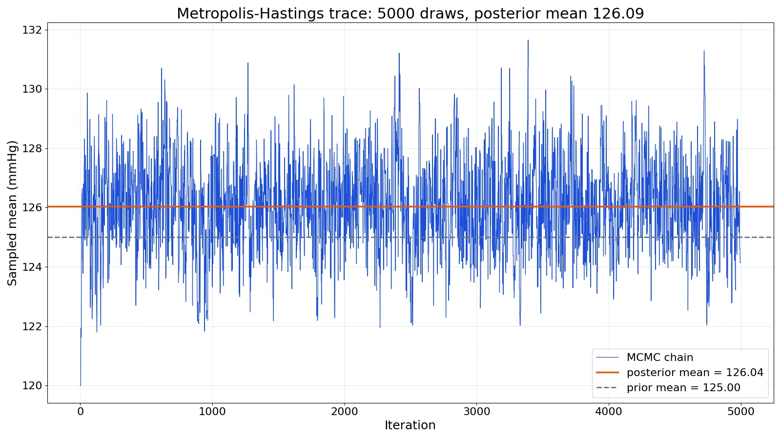
Trace plot. Plot the draws against iteration number. A healthy trace looks like a fuzzy caterpillar with no trend and no long flat stretches. The figure for this run shows the chain settling near the analytic posterior mean of 126.04 mmHg, well above the prior mean of 125.00 mmHg.
Acceptance rate. Too high means the chain is crawling and will take forever to explore. Too low means it is stuck. For a normal proposal in low dimensions, something near 0.4 to 0.6 is a reasonable target.

The key point is that the draws are correlated with each other, so the effective sample size is smaller than the raw count of 4,000 post-burn-in draws. Treat the posterior standard deviation as an estimate, not an exact figure.

When to Use It (and when not to)

Use MCMC when the posterior has no closed form. That covers most realistic Bayesian models: hierarchical models with group-level parameters, models with latent variables, and anything where the normalizing constant is an integral you cannot evaluate. It is also the standard tool when you need the full posterior rather than a point estimate, since it gives you the whole distribution for free. If you are still deciding between a point estimate and a full posterior, Maximum Likelihood Estimation: Definition and Example covers the frequentist alternative.

Do not use MCMC when a closed form exists. In the example above, the conjugate normal-normal update gives the exact answer in three lines, and running a sampler would only add noise. Do not use it when you need a single fast estimate and a simpler method will do. Do not use it when your model has hundreds of thousands of parameters and you have no gradient information, since plain Metropolis will be too slow. And do not use it without checking convergence, because a chain that has not converged produces confident-looking numbers that are simply wrong.

If you are new to simulation-based methods, Monte Carlo Simulation: Definition, Steps and Example is a gentler starting point, and What Is a Bayesian Model? Definition and Examples sets up the posterior you are sampling from.

Markov Chain Monte Carlo vs Monte Carlo Simulation

These two terms get confused constantly. Plain Monte Carlo draws independent samples from a distribution you already know how to sample from. MCMC draws dependent samples from a distribution you can only evaluate.

Feature	Monte Carlo simulation	Markov Chain Monte Carlo
Sample independence	Independent draws	Correlated draws
Requirement	You can sample directly	You can evaluate the density up to a constant
Typical use	Estimating integrals, risk simulation	Bayesian posterior inference
Main tuning knob	Number of draws	Proposal width and burn-in
Convergence check	Standard error shrinks as $1/\sqrt{N}$	Trace plots, acceptance rate, effective sample size

The practical difference is that Monte Carlo gives you a clean standard error from the sample size alone, while MCMC gives you a standard error that depends on how correlated the chain is. A chain of 5,000 draws might carry the information of only a few hundred independent draws.

Common Mistakes

Skipping burn-in. Early draws reflect the starting value, not the target. Discard them. In the example, the chain starts at 120.0 but the posterior sits near 126.0, so the earliest draws are biased low.
Reporting the raw draw count as the sample size. Correlated draws carry less information than independent ones. Compute the effective sample size before quoting a standard error.
Tuning the proposal width by acceptance rate alone. A very high acceptance rate feels good but means tiny steps and slow exploration. Check the trace plot too.
Ignoring the starting value. A chain started far from the posterior mode may take a long time to arrive. Run several chains from dispersed starting points and check they agree.
Treating the posterior mean as the answer. The mean is one summary. Report the spread and a credible interval alongside it.
Forgetting that the prior matters at small $n$. With 12 observations, the prior mean of 125.0 shifted the estimate. With 12,000 observations it would barely register.

Limitations

MCMC cannot tell you whether your model is correct. It samples from the posterior you specified, and if the likelihood or prior is wrong, the sampler will faithfully produce draws from the wrong distribution. It also cannot rescue an unidentified model, where multiple parameter values give identical likelihoods. The chain will wander and the posterior will look wide and strange, but no amount of extra iterations fixes it.

Convergence is the other hard limit. There is no test that proves a chain has converged. Diagnostics can only flag problems. A chain can appear stable for thousands of iterations and then drift to a different region, especially in multimodal posteriors where the chain gets trapped in one mode and never visits the others. Always run multiple chains and compare them. For a non-technical walkthrough of these practical issues, see Markov Chain Monte Carlo (MCMC) for Biologists.

Frequently Asked Questions

What is Markov Chain Monte Carlo in simple terms?

It is a random walk that maps out a probability distribution. You start somewhere, propose a nearby value, and move there if it looks more probable, or sometimes even if it looks less probable. After enough steps, the places the walk visits match the distribution you wanted to sample from.

Why is MCMC used for Bayesian inference?

Bayesian inference needs the posterior, which is proportional to the likelihood times the prior. The normalizing constant is usually an integral with no closed form. MCMC only needs the unnormalized product, because the constant cancels in every acceptance ratio [2].

How many iterations does MCMC need?

There is no fixed number. It depends on how correlated the draws are and how complex the posterior is. Run the chain, check the trace plot and the effective sample size, and increase the count until the estimates stabilize. In the example, 5,000 draws with 1,000 discarded as burn-in were enough for a simple one-parameter problem.

What is a good acceptance rate for the Metropolis algorithm?

For a normal random walk proposal in one or two dimensions, an acceptance rate around 0.4 to 0.6 usually mixes well. The example run accepted 3161 of 4999 proposals, a rate of 0.6323. Rates above 0.9 suggest steps that are too small, and rates below 0.1 suggest steps that are too large.

What is the difference between MCMC and Monte Carlo?

Monte Carlo draws independent samples from a distribution you can sample from directly. MCMC draws correlated samples from a distribution you can only evaluate. MCMC is what you use when direct sampling is impossible, which is the normal situation in Bayesian modeling [1].

References

- Grewal JK, Krzywinski M, Altman N (2019). Markov models, Markov chains. Nature Methods
- Puga JL, Krzywinski M, Altman N (2015). Bayesian statistics. Nature Methods
Further Reading
- NIST/SEMATECH e-Handbook of Statistical Methods
- Wasserstein RL, Lazar NA (2016). The ASA Statement on p -Values: Context, Process, and Purpose. The American Statistician
- Krzywinski M, Altman N (2013). Significance, P values and t-tests. Nature Methods
- OpenStax. Introductory Statistics 2e
Related Articles
- Monte Carlo Simulation: Definition, Steps and Example
- Probability Distributions: Definition, Types and Examples
- Bayes' Theorem: Definition, Formula and Examples
- Maximum Likelihood Estimation: Definition and Example
- Probability Density Function: Definition, Formula and Examples
- Markov Chain Monte Carlo (MCMC) for Biologists
- Poisson Distribution: Formula and Examples
- Markov State Models in Molecular Dynamics Simulations