Bayes' Theorem: Definition, Formula and Examples

By Dr. Zubair Khalid, DVM, MS, PhD · 2026-10-03

Bayes' theorem is a formula for reversing a conditional probability. If you know how likely a positive test is among sick people, the theorem tells you how likely sickness is among people who test positive. It combines a prior belief with new evidence to produce an updated probability, which is why the Bayesian theorem sits at the center of Bayesian statistics [1].

Quick Answer

Bayes' theorem computes $P(H \mid E)$, the probability of a hypothesis given evidence, from the reverse conditional probability $P(E \mid H)$.
The formula is $P(H \mid E) = \dfrac{P(E \mid H)\,P(H)}{P(E)}$.
$P(H)$ is the prior, $P(E \mid H)$ is the likelihood, $P(E)$ is the marginal probability of the evidence, and $P(H \mid E)$ is the posterior.
The posterior is a weighted compromise: strong evidence moves the prior a lot, weak evidence moves it a little [2].
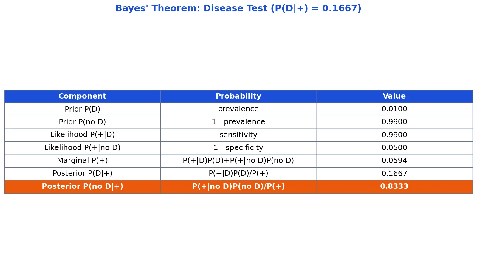
In a disease test with 1% prevalence, 99% sensitivity and 95% specificity, a positive result raises the probability of disease from 0.01 to only 0.1667.

What Bayes' Theorem Means

In plain terms, Bayes' theorem is a rule for updating what you believe after you see data. You start with a prior probability, look at how well the hypothesis predicts the data you observed, and end with a posterior probability that reflects both.

The precise definition is a relationship between conditional probabilities. For a hypothesis $H$ and evidence $E$, the probability of $H$ conditional on $E$ is the ratio of the unconditional probability of the conjunction of the hypothesis with the data to the unconditional probability of the data alone, provided both terms of that ratio exist [1]. Written out:

$$P(H \mid E) = \frac{P(H \cap E)}{P(E)}$$

Because $P(H \cap E) = P(E \mid H)\,P(H)$, this rearranges into the familiar form of the theorem. The Stanford Encyclopedia of Philosophy notes that the theorem's central insight is that a hypothesis is confirmed by any body of data that its truth renders probable [1]. That single idea is the cornerstone of subjectivist and Bayesian approaches to evidence and learning [1].

How It Works

The formula has four parts. Each one has a name and a job.

$$P(H \mid E) = \frac{P(E \mid H)\,P(H)}{P(E)}$$

Symbol	Name	Meaning
$P(H)$	Prior	Your probability for the hypothesis before seeing the evidence
$P(E \mid H)$	Likelihood	How probable the evidence is if the hypothesis is true
$P(E)$	Marginal likelihood	How probable the evidence is overall, under all hypotheses
$P(H \mid E)$	Posterior	Your updated probability for the hypothesis after the evidence

The denominator is usually the part people forget. When there are only two hypotheses, $H$ and its complement $\text{no } H$, you expand it with the law of total probability:

$$P(E) = P(E \mid H)\,P(H) + P(E \mid \text{no } H)\,P(\text{no } H)$$

That expansion is what makes the theorem usable with numbers you can actually estimate. It also explains the base rate effect: when $P(H)$ is tiny, the second term in the denominator can dominate, and the posterior stays small even after a positive result. This is the same logic behind conditional probability, where you restrict attention to a subset of outcomes.

Worked Example

The table below only illustrates the data layout, one row per patient with a disease status and a test result. The calculation itself uses the population rates given next, not these 10 rows.

patient_id	disease_status	test_result
1	D	+
2	D	+
3	no D	-
4	no D	-
5	no D	-
6	no D	-
7	no D	-
8	no D	-
9	no D	-
10	no D	-

The scenario uses a disease prevalence of 0.01, a test sensitivity of 0.99 and a specificity of 0.95. Sensitivity is $P(+ \mid D)$ and specificity is $P(- \mid \text{no } D)$, so the false positive rate is $1 - 0.95 = 0.05$.

Step 1. Set the priors. Before any test, $P(D) = 0.01$ and $P(\text{no } D) = 0.99$.

Step 2. Set the likelihoods. $P(+ \mid D) = 0.99$ and $P(+ \mid \text{no } D) = 0.05$.

Step 3. Compute the marginal probability of a positive test.

$$P(+) = 0.99 \times 0.01 + 0.05 \times 0.99 = 0.0594$$

Step 4. Apply the theorem.

$$P(D \mid +) = \frac{0.99 \times 0.01}{0.0594} = 0.1667$$

Step 5. Check the complement. $P(\text{no } D \mid +) = \dfrac{0.05 \times 0.99}{0.0594} = 0.8333$. The two posteriors sum to 1.

Here is the same calculation in Python:

prevalence = 0.01
sensitivity = 0.99
specificity = 0.95
p_pos = sensitivity*prevalence + (1-specificity)*(1-prevalence)
p_d_given_pos = sensitivity*prevalence / p_pos
print(f"P(D|+) = {p_d_given_pos:.4f}")  # 0.1667

Output:

P(D|+) = 0.1667

Quantity	Value
Prior $P(D)$	0.01
Prior $P(\text{no } D)$	0.99
Likelihood $P(+ \mid D)$	0.99
Likelihood $P(+ \mid \text{no } D)$	0.05
Marginal $P(+)$	0.0594
Posterior $P(D \mid +)$	0.1667
Posterior $P(\text{no } D \mid +)$	0.8333

How to Interpret It

The posterior of 0.1667 means that among people who test positive, about 17 in 100 actually have the disease. The other 83 are false positives. That result surprises most people, because the test looks accurate at 99% sensitivity.

The reason is the base rate. Only 1% of the population has the disease, so the small false positive rate applies to a very large healthy group. Roughly 5% of 99 healthy people produce about 5 false positives, while 99% of 1 sick person produces about 1 true positive. The positives are therefore mostly false.

This is why a Bayesian approach is useful in diagnostic testing. It lets you combine prior knowledge, such as prevalence, with the test result to produce a posterior probability rather than reading the raw accuracy as if it were the answer [3]. The same updating logic applies when you revise an estimate of a project's value after new information arrives [2].

When to Use It (and when not to)

Use Bayes' theorem when you have a prior probability and a likelihood, and you want the reverse conditional probability. Typical cases include diagnostic testing, spam filtering, and any setting where you update beliefs as data arrive [4].

Use it when the prior is meaningful and defensible. In clinical work, prevalence from a real population is a reasonable prior. In a Bayesian model, the prior is a full probability distribution over parameters, and the theorem updates that distribution into a posterior.

Do not use it when you have no basis for the prior and the result is sensitive to that choice. Do not use it as a substitute for good data collection. The theorem cannot fix a biased sample or a miscalibrated test. If your likelihoods are wrong, the posterior is wrong, and it will look just as confident as a correct one.

Bayes' Theorem vs Conditional Probability

Conditional probability is the general concept. Bayes' theorem is a specific tool for inverting it.

Aspect	Conditional probability	Bayes' theorem
What it gives	$P(A \mid B)$ directly from a defined sample space	$P(H \mid E)$ from $P(E \mid H)$ and priors
Direction	Forward, as defined	Reversed
Key inputs	Joint and marginal probabilities	Prior, likelihood, marginal likelihood
Typical use	Restricting to a subgroup	Updating beliefs with evidence
Main risk	Misreading the condition	A bad or unjustified prior

If you already know $P(A \mid B)$ and just need to state it, you do not need the theorem. You need it when the conditional you want runs opposite to the one you can estimate. The same reversal idea appears in maximum likelihood estimation, which asks which parameter value makes the observed data most probable.

Common Mistakes

Ignoring the base rate. Treating a 99% sensitive test as 99% accurate for a positive patient. Fix: always include $P(H)$ in the denominator.
Confusing $P(E \mid H)$ with $P(H \mid E)$. These are different numbers. Fix: write both out in symbols before plugging in values.
Forgetting the second term in the denominator. Using only $P(E \mid H)P(H)$ understates $P(E)$. Fix: expand $P(E)$ with the law of total probability.
Using a prior you cannot defend. A convenient prior can drive the posterior. Fix: state where the prior comes from and test sensitivity to it.
Dropping the complement check. Posteriors over all hypotheses must sum to 1. Fix: compute the complement and confirm it adds up.
Treating the posterior as final truth. It is a probability given the inputs, not a verdict. Fix: report it with the assumptions behind it.

Limitations

Bayes' theorem is exact given its inputs, but the inputs are estimates. The prior and the likelihoods come from data, expert judgment, or both, and each carries uncertainty that the formula does not represent. A posterior of 0.1667 is only as good as the 0.01 prevalence and the 0.99 sensitivity you fed it.

The theorem also scales poorly by hand. With two hypotheses it is a short calculation. With many parameters you need numerical methods such as Markov chain Monte Carlo to approximate the posterior, because the denominator becomes an integral over the whole parameter space. Finally, the theorem says nothing about causation. It updates probabilities, and a strong posterior is not evidence that one variable causes another.

Frequently Asked Questions

What is Bayes' theorem in simple terms?

It is a formula for updating a probability when new evidence arrives. You multiply your prior belief by how likely the evidence is under that belief, then divide by how likely the evidence is overall. The result is your updated belief, called the posterior.

What is the difference between prior and posterior?

The prior is your probability before seeing the data. The posterior is your probability after seeing the data. In the disease example, the prior for disease is 0.01 and the posterior after a positive test is 0.1667.

Why does a positive test not mean you have the disease?

Because the test also fires on healthy people. When the disease is rare, false positives from the large healthy group outnumber true positives from the small sick group. That is why the posterior stays low even with a highly sensitive test.

Can Bayes' theorem be used with more than two hypotheses?

Yes. Replace the two-term denominator with a sum over all hypotheses: $P(E) = \sum_i P(E \mid H_i)\,P(H_i)$. The posterior for each hypothesis is then its own likelihood times prior, divided by that sum. This is the form used in naive Bayes classifiers.

What does the denominator in Bayes' theorem represent?

It is the total probability of the evidence under all possible hypotheses. It acts as a normalizing constant, scaling the numerator so the posteriors sum to 1. You compute it with the law of total probability.

References

- Bayes’ Theorem (Stanford Encyclopedia of Philosophy/Spring 2021 Edition)
- Bayes Theorem Supplement
- Thi Mai H, He S, Alexandrou E, Alfred Frost S. (2022). An introduction to Bayes' theorem and examples of its application to a diagnostic test and a clinical trial. Nurse researcher
- Rindskopf D. (2020). Overview of Bayesian Statistics. Evaluation review
Further Reading
- 20.2: Bayes’ Theorem and Inverse Inference - Statistics LibreTexts/20%3A_Bayesian_Statistics/20.02%3A_Bayes_Theorem_and_Inverse_Inference)
- NIST/SEMATECH e-Handbook of Statistical Methods
Related Articles
- Bayesian Classifiers: How Naive Bayes Works
- What Is a Bayesian Model? Definition and Examples
- Maximum Likelihood Estimation: Definition and Example
- Markov Chain Monte Carlo: Definition and Examples
- Probability Distributions: Definition, Types and Examples
- Bayes theorem biology examples
- MAP and TAU in Bayesian Statistics
- Bayesian Hypothesis Testing for Biological Data