Bayesian Classifiers: How Naive Bayes Works
By Dr. Zubair Khalid, DVM, MS, PhD ·
Bayesian classifiers are probabilistic models that assign a label to a data point by combining how common each class is with how likely the observed features are under each class. The most widely used member of this family is the naive Bayes classifier, which applies Bayes' theorem and assumes that features are independent given the class. That assumption is usually false, yet the method still performs well on tasks like spam filtering and document classification [1][2].
Quick Answer
- A Bayesian classifier picks the class with the highest posterior probability $P(y \mid x)$, computed from a prior $P(y)$ and feature likelihoods $P(x_i \mid y)$ [1].
- Naive Bayes assumes features are conditionally independent given the class, so the joint likelihood becomes a product of per-feature probabilities [2].
- The "naive" independence assumption is rarely true, but the classifier often works well anyway, especially for text [2][3].
- Different variants (Multinomial, Bernoulli, Gaussian) differ only in how they model $P(x_i \mid y)$ [1].
- Training is fast and needs little data because you only estimate counts or simple distribution parameters [1].
What Bayesian Classifiers Mean
In plain terms, a Bayesian classifier asks: given what I see, which class is most probable? It answers with probabilities, not just a label, so you can see how confident the model is.
The precise definition starts with Bayes' theorem. For a class $y$ and a feature vector $x = (x_1, \dots, x_n)$:
$$P(y \mid x) = \frac{P(y)\,P(x \mid y)}{P(x)}$$
Because $P(x)$ is the same for every class, it does not affect which class wins. The classifier therefore uses maximum a posteriori (MAP) estimation and picks the class that maximizes the numerator [1]:
$$\hat{y} = \arg\max_y P(y) \prod_{i=1}^{n} P(x_i \mid y)$$
The product appears because naive Bayes assumes the features are independent given the label, so $P(x \mid y) = \prod_{i=1}^{n} P(x_i \mid y)$ [2]. This is the "naive" step. For spam filtering, it means treating each word as if it appeared independently of every other word, which is clearly untrue, yet the resulting classifiers still work well in practice [2].
One clarification that surprises many people: naive Bayes is named after Bayes' theorem but is not a fully Bayesian method. It estimates parameters from data by likelihood, so it is closer to a frequentist classifier that happens to use Bayes' rule for prediction [3][4]. If you want the broader picture, see What Is a Bayesian Model? Definition and Examples.
How It Works
Training a naive Bayes classifier means estimating two things from your labeled data.
The priors. $P(y)$ is the relative frequency of each class in the training set [1]. With 5 spam and 5 non-spam emails, each prior is 0.5.
The conditional probabilities. $P(x_i \mid y)$ is how likely feature $i$ is within class $y$. For word counts, this is the count of that word in the class divided by the total word count in the class. The variants of naive Bayes differ mainly in the distribution they assume for $P(x_i \mid y)$ [1]:
| Variant | Feature type | Models $P(x_i \mid y)$ as |
|---|---|---|
| MultinomialNB | Word or event counts | Multinomial distribution |
| BernoulliNB | Binary present/absent features | Bernoulli distribution [1] |
| GaussianNB | Continuous features | Normal distribution |
Smoothing. If a word never appears in a class, its conditional probability is zero, and one zero wipes out the whole product. Laplace smoothing adds a small count $\alpha$ to every feature so no probability is exactly zero. In scikit-learn this is the alpha parameter, and alpha=1 is the default form of additive smoothing [1].
Prediction. At test time you multiply the prior by the conditional probabilities for the observed features, once per class, and pick the largest. In practice you sum logarithms instead of multiplying, because many small probabilities underflow floating-point numbers. The $\arg\max$ is unchanged since the logarithm is monotonic.
Worked Example
The dataset is 10 emails labeled spam or not spam, with counts of the words "free" and "meeting."
| id | free | meeting | label |
|---|---|---|---|
| E01 | 3 | 0 | spam |
| E02 | 2 | 0 | spam |
| E03 | 4 | 1 | spam |
| E04 | 1 | 0 | spam |
| E05 | 2 | 1 | spam |
| E06 | 0 | 3 | not spam |
| E07 | 0 | 2 | not spam |
| E08 | 1 | 4 | not spam |
| E09 | 0 | 2 | not spam |
| E10 | 0 | 3 | not spam |
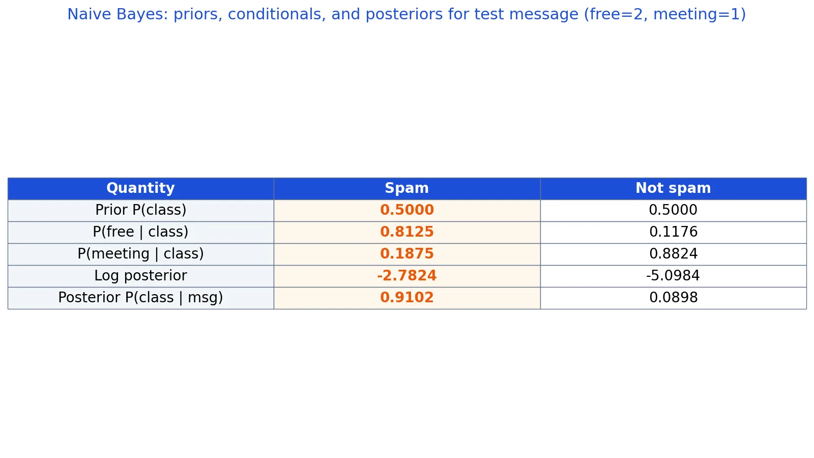
Step 1: priors. 5 of 10 emails are spam, so $P(\text{spam}) = 5/10 = 0.5000$ and $P(\text{not spam}) = 5/10 = 0.5000$.
Step 2: total word counts per class. The spam emails contain 14 words in total. The not-spam emails contain 15.
Step 3: conditional probabilities with Laplace smoothing ($\alpha = 1$). The denominator adds $\alpha$ times the number of distinct words (2), so it becomes total + 2.
- $P(\text{free} \mid \text{spam}) = (12+1)/(14+2) = 0.8125$
- $P(\text{meeting} \mid \text{spam}) = (2+1)/(14+2) = 0.1875$
- $P(\text{free} \mid \text{not spam}) = (1+1)/(15+2) = 0.1176$
- $P(\text{meeting} \mid \text{not spam}) = (14+1)/(15+2) = 0.8824$
Step 4: score a test message with free = 2 and meeting = 1. Working in logs:
$$\ln(0.5000) + 2\ln(0.8125) + 1\ln(0.1875) = -2.7824 \quad (\text{spam})$$ $$\ln(0.5000) + 2\ln(0.1176) + 1\ln(0.8824) = -5.0984 \quad (\text{not spam})$$
Step 5: normalize. Converting the log scores back to probabilities gives $P(\text{spam} \mid \text{message}) = 0.9102$ and $P(\text{not spam} \mid \text{message}) = 0.0898$. The predicted class is spam.
The same result in scikit-learn:
from sklearn.naive_bayes import MultinomialNB
import numpy as np
X = np.array([[3,0],[2,0],[4,1],[1,0],[2,1],[0,3],[0,2],[1,4],[0,2],[0,3]])
y = np.array(['spam']*5 + ['not spam']*5)
clf = MultinomialNB(alpha=1).fit(X, y)
proba = clf.predict_proba([[2,1]])[0]  # classes_ sorted: ['not spam', 'spam']
print(f"P(not spam | message) = {proba[0]:.4f}")
print(f"P(spam | message)     = {proba[1]:.4f}")
print(f"predicted class       = {clf.predict([[2,1]])[0]}")
Output:
P(not spam | message) = 0.0898
P(spam | message)     = 0.9102
predicted class       = spam
The word "free" appears twice, and "free" is far more common in spam, so the evidence pushes hard toward spam even though "meeting" points the other way.
How to Interpret It
The output is a probability per class, and the prediction is simply the largest one. Read the gap between the top two probabilities as a rough measure of confidence. In the example, 0.9102 against 0.0898 is a decisive call. A split like 0.51 against 0.49 is barely better than a coin flip, and you should treat such predictions with caution.
The conditional probabilities are also readable on their own. $P(\text{free} \mid \text{spam}) = 0.8125$ means that in the spam class, "free" accounts for about 81 percent of word occurrences. That is a direct, interpretable statement about the data, which is one reason naive Bayes stays popular for text. For a wider view of how models like this fit together, see Introduction To Statistical Learning.
When to Use It (and when not to)
Use naive Bayes when you have text or count data, when you need a fast baseline, or when labeled data is scarce. It requires only a small amount of training data to estimate its parameters, and it can be extremely fast compared to more complex models [1]. Spam filtering and document classification are its classic successes [1][2].
Avoid it when features are strongly correlated and those correlations carry the signal. If two features always move together, naive Bayes double-counts the evidence and becomes overconfident. It is also a poor fit when you need well-calibrated probabilities or when the decision boundary is highly non-linear in a way the assumed distribution cannot capture. For those cases, compare against K-Nearest Neighbors (KNN): Algorithm and Examples or Support Vector Machines (SVM): Definition and Examples.
Naive Bayes vs Logistic Regression
Logistic regression is the closest relative. Both are linear classifiers in the log-odds sense, and when the naive Bayes assumption actually holds, the two produce asymptotically the same model [2]. The difference is how they learn.
| Aspect | Naive Bayes | Logistic Regression |
|---|---|---|
| What it models | $P(x \mid y)$ and $P(y)$, then applies Bayes' rule | $P(y \mid x)$ directly |
| Assumption | Features independent given the class [2] | None about feature independence |
| Data needs | Works with small samples [1] | Needs more data to fit weights |
| Speed | Very fast to train [1] | Slower, iterative fitting |
| Calibration | Often overconfident | Usually better calibrated |
If you have plenty of data and correlated features, logistic regression is often the safer choice. If you have little data and need speed, naive Bayes is hard to beat.
Common Mistakes
- Forgetting smoothing. A single zero conditional probability zeroes the entire product. Fix it by adding Laplace smoothing, for example
alpha=1in scikit-learn [1]. - Multiplying raw probabilities. Long feature vectors underflow to zero. Fix it by summing log probabilities instead.
- Using MultinomialNB on binary data. If your features are only present or absent, BernoulliNB models them correctly [1]. MultinomialNB expects counts.
- Believing the independence assumption. The features are almost never independent [2]. The method works despite this, so do not reject it on that ground alone, but do not trust its probability magnitudes either.
- Treating it as a fully Bayesian method. Naive Bayes estimates parameters by likelihood, so it is not Bayesian inference in the strict sense [3][4].
- Ignoring class imbalance. Priors come straight from class frequencies, so a rare class gets a small prior. Check the priors before trusting the output.
Limitations
Naive Bayes cannot model interactions between features. If the meaning of one feature depends on another, the classifier will miss it, and its probability estimates will be too extreme in both directions. The predicted label is often right even when the probability is overstated, which makes the scores misleading if you use them for ranking or thresholding.
It also assumes a specific distribution for each feature, and a wrong choice hurts accuracy. MultinomialNB on continuous measurements or GaussianNB on skewed counts will underperform. The model is a strong baseline, not a final answer, and it should be compared against alternatives on your own data. For help setting up that comparison, see Python for Machine Learning: A Beginner's Guide.
Frequently Asked Questions
Why is it called naive Bayes?
It is called naive because of the independence assumption. The model treats every feature as independent of the others given the class, which is a bold and usually false simplification [2]. The name Bayes comes from its use of Bayes' theorem to combine the prior with the likelihoods [3].
Is naive Bayes actually a Bayesian method?
Not in the strict sense. It uses Bayes' theorem for prediction, but it estimates its parameters from data by maximum likelihood instead of placing prior distributions over them [3][4]. That places it closer to frequentist statistics than to full Bayesian inference.
What is the difference between Multinomial, Bernoulli and Gaussian naive Bayes?
They differ only in the assumed distribution of $P(x_i \mid y)$ [1]. MultinomialNB suits word counts, BernoulliNB suits binary present-or-absent features, and GaussianNB suits continuous features modeled with a normal distribution. Pick the one that matches your data type.
Does naive Bayes need a lot of training data?
No. It needs only a small amount of data to estimate the necessary parameters, which is one of its main advantages [1]. That makes it a good choice for small datasets and quick baselines.
Can naive Bayes handle more than two classes?
Yes. The formula generalizes to any number of classes, and the classifier simply picks the class with the highest posterior. The spam example uses two classes, but the same $\arg\max$ over $P(y) \prod P(x_i \mid y)$ applies to as many classes as you have [1].
References
- 1.9. Naive Bayes, scikit-learn 1.9.1 documentation
- Lecture 5: Bayes Classifier and Naive Bayes
- Naïve Bayes, ACME Labs
- Naive Bayes | CAIS++
Further Reading
- Naive Bayes Classifiers
- Lever J, Krzywinski M, Altman N (2016). Classification evaluation. Nature Methods
Related Articles
- Bayes' Theorem: Definition, Formula and Examples
- Python for Machine Learning: A Beginner's Guide
- K-Nearest Neighbors (KNN): Algorithm and Examples
- What Is Random Forest? Algorithm and Examples
- Support Vector Machines (SVM): Definition and Examples
- Introduction To Statistical Learning
- MAP and TAU in Bayesian Statistics
- Elements Of Statistical Learning