Types of Data: Nominal, Ordinal, Interval, Ratio

By Dr. Zubair Khalid, DVM, MS, PhD · 2026-10-03

The four main types of data are nominal, ordinal, interval and ratio. Each type is a level of measurement, and the level decides what you can legitimately do with the values. Pick the wrong type and you will compute averages that mean nothing or draw charts that mislead.

Quick Answer

Nominal data are category names with no order. You can compare equality only, so the mode and frequency counts are your main tools [1].
Ordinal data are ordered categories where the gaps between ranks are not equal. Medians and percentiles work, means usually do not.
Interval data are numeric with equal gaps but an arbitrary zero. Addition and subtraction are valid, ratios are not.
Ratio data are numeric with equal gaps and a true zero. Every arithmetic operation, including ratios and coefficients of variation, is valid.
The levels form a hierarchy. Ratio data support interval, ordinal and nominal comparisons, but nominal data support only equality [1].

What Type of Data Means

In plain terms, the type of data is the answer to one question: what comparisons do these values support? A column of country names and a column of incomes are both "data," but they allow completely different operations.

The precise statistical definition comes from measurement theory. A level of measurement describes the structure of the mapping from a real-world property to recorded values. Nominal measurement preserves only identity. Ordinal measurement preserves identity and order. Interval measurement preserves identity, order and equal distances. Ratio measurement preserves all of that plus a meaningful zero point.

This is why the type of data is not a property of the numbers themselves. It is a property of how you interpret them. A field stored as an integer can still be nominal, ordinal or quantitative depending on the question you ask [1]. Ages recorded as 10, 20 and 30 could be treated as nominal (underage or overage), ordinal (grouped by year) or quantitative (average age) [1].

How It Works

Each level permits a specific set of operations. The table below summarizes the mechanism.

Level	Order	Equal gaps	True zero	Valid central tendency	Valid spread
Nominal	No	No	No	Mode	Frequency counts
Ordinal	Yes	No	No	Median	Range, IQR
Interval	Yes	Yes	No	Mean, median, mode	SD, variance, range
Ratio	Yes	Yes	Yes	Mean, median, mode, geometric mean	SD, variance, CV, ratios

The arithmetic behind the two numeric levels is where the distinction bites. For interval data, the mean is defined as

$$\bar{x} = \frac{1}{n}\sum_{i=1}^{n} x_i$$

where $x_i$ are the observed values and $n$ is the number of observations. This formula is valid for interval and ratio data. It is not valid for nominal data, and it is questionable for ordinal data because the spacing between ranks is unknown.

The sample standard deviation uses $n-1$ in the denominator:

$$s = \sqrt{\frac{\sum_{i=1}^{n}(x_i - \bar{x})^2}{n-1}}$$

where $s$ is the sample standard deviation, $x_i$ is each value, $\bar{x}$ is the sample mean and $n$ is the sample size. The coefficient of variation is the ratio of the two:

$$CV = \frac{s}{\bar{x}}$$

The CV only makes sense for ratio data. It requires a true zero, because dividing by a mean that sits on an arbitrary scale produces a meaningless number. Temperature in Celsius has no true zero, so a CV of temperature is not interpretable. Income has a true zero, so its CV is meaningful.

Worked Example

The dataset is a 10-row survey recording eye colour, satisfaction on a 1 to 5 scale, temperature in Celsius and income in USD.

id	eye_colour	satisfaction	temperature_C	income_USD
P01	Blue	5	21.5	42000
P02	Brown	4	22.1	51500
P03	Green	3	19.8	38000
P04	Blue	5	23.4	62000
P05	Hazel	2	20.2	47000
P06	Brown	4	24.0	55000
P07	Green	1	18.5	33500
P08	Blue	5	22.7	58000
P09	Hazel	3	21.0	44500
P10	Brown	2	20.5	49000

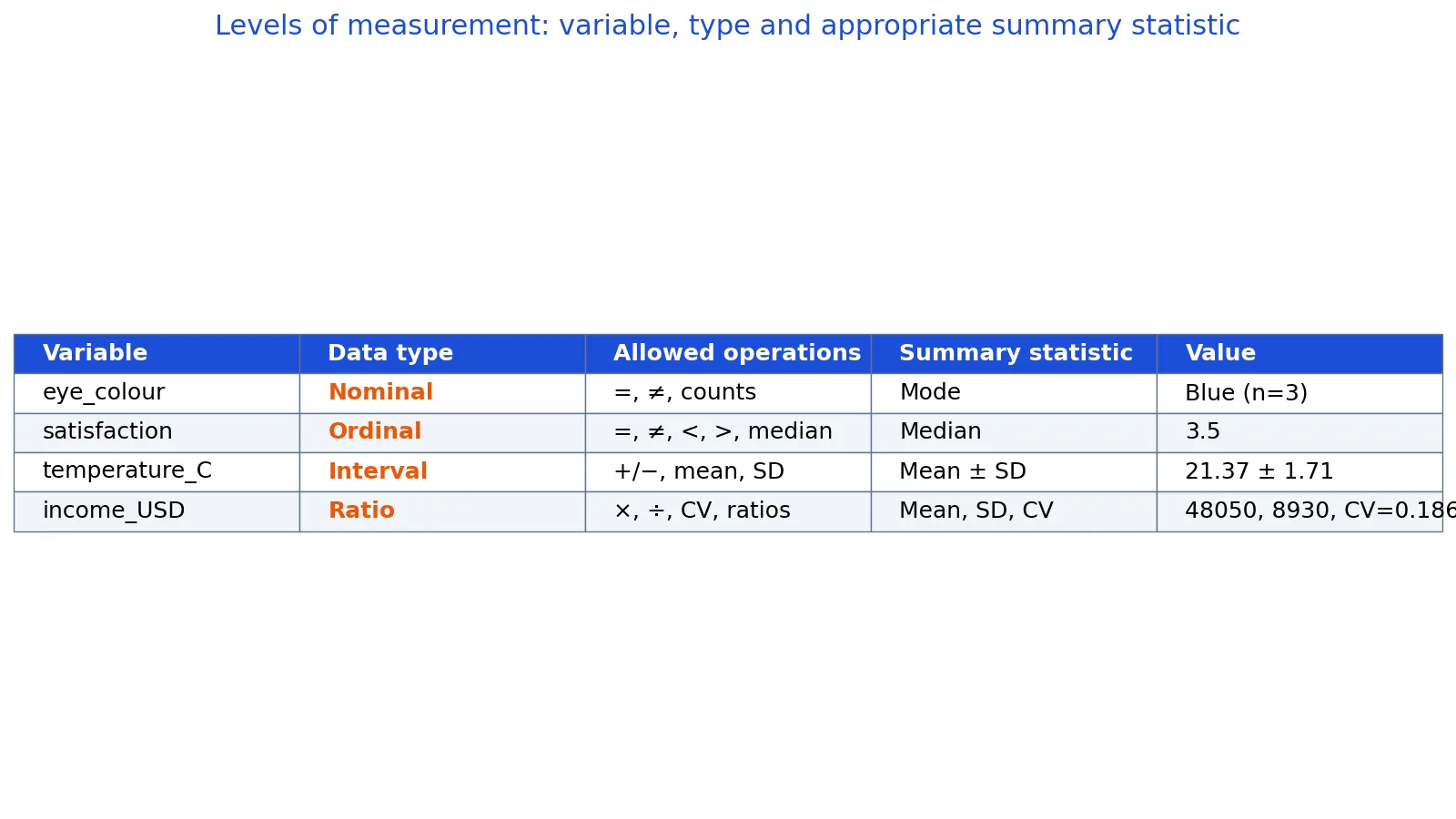
Nominal (eye colour). The only valid summary is the mode and the counts. The counts are Blue 3, Brown 3, Green 2, Hazel 2. Blue and Brown tie with n=3 each, so the variable is bimodal with modes Blue and Brown. A mean of eye colour does not exist.

Ordinal (satisfaction). The sorted values are 1, 2, 2, 3, 3, 4, 4, 5, 5, 5. With n=10, the median is the average of the 5th and 6th values: (3+4)/2 = 3.5. The median is the right summary here because the distance between "1" and "2" is not guaranteed to equal the distance between "4" and "5."

Interval (temperature). The sum is 213.7 and n=10, so the mean is 213.7/10 = 21.3700. The sample standard deviation is 1.7101. The minimum is 18.5 and the maximum is 24. You can say 21.37 °C is warmer than 20 °C, but you cannot say 21.37 °C is "twice as warm" as 10.685 °C.

Ratio (income). The sum is 480500, so the mean is 48050.0000. The sample standard deviation is 8930.1300. The coefficient of variation is 8930.1300/48050.0000 = 0.1859. The minimum is 33500 and the maximum is 62000. Here ratios are valid: the highest income is about 1.85 times the lowest.

The same operations are available in a spreadsheet. MEDIAN on the satisfaction column returns 3.5. STDEV.S on temperature returns 1.7101 and on income returns 8930.1300. MODE works only on numbers, so on the eye colour text it returns #N/A. Use COUNTIF for each colour instead, which shows Blue and Brown tied at 3.

A SQL group-by on eye colour returns two columns and four rows: ('Blue', 3), ('Brown', 3), ('Green', 2), ('Hazel', 2).

import pandas as pd, statistics
df = pd.DataFrame({
    'eye_colour': ['Blue','Brown','Green','Blue','Hazel','Brown','Green','Blue','Hazel','Brown'],
    'satisfaction': [5,4,3,5,2,4,1,5,3,2],
    'temperature_C': [21.5,22.1,19.8,23.4,20.2,24.0,18.5,22.7,21.0,20.5],
    'income_USD': [42000,51500,38000,62000,47000,55000,33500,58000,44500,49000],
})
print(df['eye_colour'].mode()[0])          # Blue (mode() returns Blue and Brown, [0] takes the first)
print(statistics.median(df['satisfaction']))  # 3.5
print(statistics.mean(df['temperature_C']))   # 21.3700
print(statistics.stdev(df['temperature_C']))  # 1.7101
print(statistics.mean(df['income_USD']))      # 48050.0000
print(statistics.stdev(df['income_USD']))     # 8930.1300

Output:

Blue
3.5
21.37
1.7101331981911685
48050
8930.130022694084

How to Interpret It

Read the level of measurement before you read any statistic. If a reported mean comes from ordinal data, treat it as a rough summary at best. If a reported ratio comes from interval data, the ratio is not meaningful.

For nominal data, interpret the mode as the most frequent category and the counts as the distribution. For ordinal data, interpret the median as the middle rank and the interquartile range as the spread of the middle half. For interval data, interpret the mean and standard deviation as location and spread on a scale whose zero is a convention. For ratio data, interpret the mean, standard deviation and CV together, because the CV tells you how large the spread is relative to the typical value.

The hierarchy matters when you choose a chart. Nominal data suit bar charts of counts. Ordinal data suit ordered bar charts or dot plots. Interval and ratio data suit histograms, box plots and scatter plots. The encoding choices follow directly from the comparisons the data support [1].

When to Use It (and when not to)

Use the nominal label when values are names or labels with no inherent order, such as eye colour, country or blood type. Use ordinal when the categories have a clear direction but uneven spacing, such as satisfaction ratings, education levels or pain scales. Use interval when differences are meaningful but zero is arbitrary, such as temperature in Celsius or Fahrenheit, calendar years or standardized test scores. Use ratio when zero means "none," such as income, height, weight, counts and duration.

Do not use the numeric label just because the column contains digits. ZIP codes, phone numbers and jersey numbers are nominal. Do not compute a mean for a nominal variable. Do not compute a coefficient of variation for an interval variable. Do not assume that a Likert scale is interval just because it is coded 1 to 5. Treat it as ordinal unless you have evidence that respondents perceive the gaps as equal.

Nominal vs Ordinal

These two are the most commonly confused, because both involve categories.

Feature	Nominal	Ordinal
Order	None	Meaningful
Example	Eye colour	Satisfaction 1 to 5
Equality comparison	Yes	Yes
Rank comparison	No	Yes
Best central tendency	Mode	Median
Best spread measure	Counts	Range, IQR
Typical chart	Bar chart of counts	Ordered bar chart

The practical test is simple. Ask whether one category is genuinely "more" than another. If yes, the variable is ordinal. If the categories are interchangeable labels, it is nominal.

Common Mistakes

Averaging nominal codes. Assigning 1 to Blue and 2 to Brown and computing a mean produces a number with no meaning. Use counts and the mode instead.
Treating ordinal scales as interval. Summing Likert items into a total score assumes equal gaps that the scale does not guarantee. Report medians, or use methods designed for ordinal data.
Computing ratios on interval data. Saying 40 °C is "twice as hot" as 20 °C is wrong because 0 °C is not an absence of temperature. Ratios require a true zero.
Assuming a numeric column is ratio. A year, a rating and a count all look numeric but behave differently. Check the zero point and the spacing before choosing statistics.
Using the coefficient of variation on interval data. The CV divides by the mean, so it needs a true zero. On Celsius temperatures the result changes if you switch to Fahrenheit.
Ignoring the hierarchy when combining variables. Mixing a nominal predictor with a ratio outcome is fine, but the analysis method must respect each variable's level.

Limitations

The four-level framework is a useful simplification, not a complete theory. Real scales often sit between levels. A Likert scale is ordinal by construction but is frequently analyzed as interval in practice, and the results can differ. Some variables change level depending on the question, as the age example shows [1].

The framework also says nothing about sampling, measurement error or study design. A perfectly identified ratio variable measured badly still produces bad statistics. Level of measurement tells you which operations are defensible, not whether your data are any good.

Frequently Asked Questions

What is the difference between interval and ratio data?

Interval data have equal gaps but an arbitrary zero, so differences are meaningful and ratios are not. Ratio data have equal gaps and a true zero, so both differences and ratios are meaningful. Temperature in Celsius is interval. Income in dollars is ratio.

Can I calculate a mean for ordinal data?

You can calculate it, but the result is often hard to defend because the gaps between ranks are unknown. The median is the safer summary. If you need a mean, state the assumption that the scale is approximately interval and check whether conclusions change under a median-based analysis.

Is a Likert scale nominal, ordinal or interval?

A single Likert item is ordinal. The response categories have a clear order but the psychological distance between "agree" and "strongly agree" is not guaranteed to equal the distance between "neutral" and "agree." Many researchers treat summed multi-item scales as interval, which is a modeling choice worth stating explicitly.

Why does the type of data change which chart I should use?

Because a chart encodes comparisons. A bar chart of counts shows equality comparisons, which suits nominal data. A histogram shows the shape of a distribution, which requires equal gaps. Choosing a chart that implies order or equal spacing your data do not have will mislead readers [1].

What type of data is a count?

Counts are ratio data. Zero means no occurrences, the gaps between consecutive counts are equal, and ratios are meaningful. You can say one group has twice as many events as another.

References

Data Types, Graphical Marks, and Visual Encoding Channels - Visualization Curriculum

References

Further Reading
- 4.2: Data Types - Chemistry LibreTexts
- Wilson G, Bryan J, Cranston K et al. (2017). Good enough practices in scientific computing. PLOS Computational Biology
- Wilkinson MD, Dumontier M, Aalbersberg IJ et al. (2016). The FAIR Guiding Principles for scientific data management and stewardship. Scientific Data
- NIST/SEMATECH e-Handbook of Statistical Methods
- Broman KW, Woo KH (2018). Data Organization in Spreadsheets. The American Statistician
Related Articles
- Levels of Measurement: Nominal, Ordinal, Interval and Ratio
- What Is Ordinal Data? Definition and Examples
- What Is a Nominal Variable? Definition and Examples
- Interval Data: Definition, Examples and When to Use It
- Nominal vs Ordinal Variables: Differences and Examples
- Types Of Statistical Analysis
- How to Choose the Right Chart Type for Your Research Data
- Statistical Synonyms: A Guide to Terminology in Statistics