Interval Data: Definition, Examples and When to Use It

By Dr. Zubair Khalid, DVM, MS, PhD · 2026-10-03

Interval data is numeric data where the distance between any two adjacent values is equal, but zero does not mean "none." Temperature in Celsius, calendar years, and IQ scores are common examples. Because the scale has equal intervals, you can add and subtract values meaningfully, but because zero is arbitrary, ratios and percentages are not meaningful.

Quick Answer

Interval data has equal, meaningful distances between consecutive values, so a difference of 5 points means the same thing anywhere on the scale.
Zero is arbitrary, not absolute. 0°C does not mean "no temperature," so 20°C is not "twice as hot" as 10°C.
Valid statistics include the mean, median, mode, standard deviation, range, and correlation.
Invalid operations include ratios, percentages of a total, and geometric means, because they assume a true zero.
The classic test: differences stay consistent when you change units, but ratios change. That is the signature of interval data.

What Interval Data Means

In plain terms, interval data is a measurement scale where the gaps between values are equal and meaningful, but the starting point is a matter of convention. You can say one value is 5 units higher than another. You cannot say one value is twice another.

The precise statistical definition: interval data is a level of measurement in which the mapping from the empirical system to the numeric system preserves order and the equality of intervals, but not the equality of ratios. In formal terms, if $x$ and $y$ are two values, then $x - y$ is meaningful, but $x / y$ is not, because the scale is unique only up to a positive affine transformation:

$$x' = a x + b, \quad a > 0$$

That means you can multiply every value by a positive constant and add a constant, and the scale still carries the same information. Celsius to Fahrenheit is exactly this transformation, with $a = 9/5$ and $b = 32$. The differences survive the change. The ratios do not.

This is what separates interval data from ordinal data, where you know only the order, and from ratio data, where a true zero makes ratios meaningful. If you want the full picture of all four levels, see types of data: nominal, ordinal, interval, ratio.

How It Works

The mechanism is simple. Interval scales preserve two things and lose one.

Preserved: order. If $x > y$, the measurement reflects a genuinely higher quantity.

Preserved: equal intervals. The difference $x - y$ is comparable across the whole scale. The gap between 5 and 8 equals the gap between 30 and 33.

Lost: ratios. The quantity $x / y$ depends on where zero sits, so it is not stable.

For a temperature scale, the conversion is:

$$F = \frac{9}{5}C + 32$$

where $C$ is the temperature in Celsius and $F$ is the temperature in Fahrenheit. The multiplier $\frac{9}{5}$ stretches the intervals. The offset $32$ shifts the zero point. Because the offset is not zero, ratios computed in Celsius and Fahrenheit disagree.

The same logic applies to any interval variable. Standard deviation scales by the same factor $a$, so it changes when you change units, but it changes in a predictable, proportional way. The mean shifts by $b$ and scales by $a$. Both are still valid summaries because they depend only on order and intervals.

Worked Example

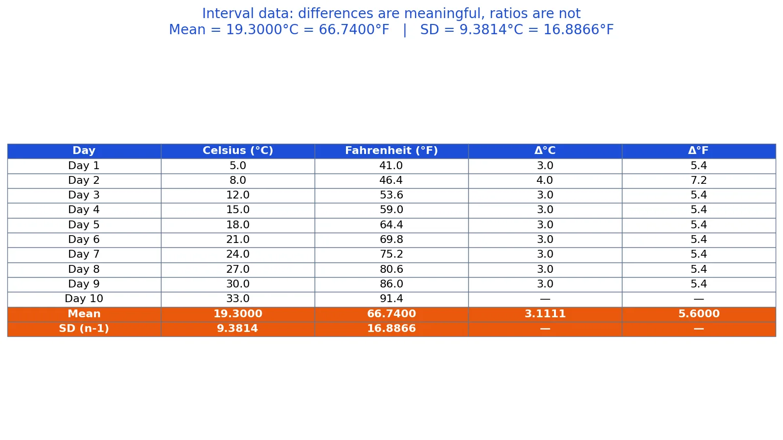
Here is a dataset of 10 days of daily temperature, recorded in both Celsius and Fahrenheit.

Day	Celsius	Fahrenheit
Day 1	5	41
Day 2	8	46.4
Day 3	12	53.6
Day 4	15	59
Day 5	18	64.4
Day 6	21	69.8
Day 7	24	75.2
Day 8	27	80.6
Day 9	30	86
Day 10	33	91.4

Step 1: Confirm the intervals are equal. The consecutive differences in Celsius are 3.0, 4.0, 3.0, 3.0, 3.0, 3.0, 3.0, 3.0, 3.0. The consecutive differences in Fahrenheit are 5.4, 7.2, 5.4, 5.4, 5.4, 5.4, 5.4, 5.4, 5.4. Each Celsius gap of 3.0 maps to a Fahrenheit gap of 5.4, and the 4.0 gap maps to 7.2. The intervals match after the $\frac{9}{5}$ scaling. This is the defining property of interval data.

Step 2: Compute the mean. The Celsius values sum to 193.0, so the mean is $193.0 / 10 = 19.3000$. The Fahrenheit values sum to 667.4, so the mean is $667.4 / 10 = 66.7400$. Both means are valid summaries.

Step 3: Compute the standard deviation. The sample standard deviation (n-1) is 9.3814 for Celsius and 16.8866 for Fahrenheit. The ratio of the two SDs is $16.8866 / 9.3814 = 1.8$, which equals $\frac{9}{5}$. The spread scales exactly with the unit change.

Step 4: Test the ratio. Take 24°C and 5°C. The ratio is $24.0 / 5.0 = 4.8000$. Now take the same two days in Fahrenheit: 75.2°F and 41°F. The ratio is $75.2 / 41.0 = 1.8341$. The two ratios disagree. That disagreement is the proof that temperature is interval, not ratio. If the scale had a true zero, the ratios would match.

Here is the Python code that produces these values:

import statistics
celsius = [5.0, 8.0, 12.0, 15.0, 18.0, 21.0, 24.0, 27.0, 30.0, 33.0]
fahrenheit = [c*9/5+32 for c in celsius]
mean_c = statistics.mean(celsius)   # 19.3000
sd_c   = statistics.stdev(celsius)  # 9.3814
mean_f = statistics.mean(fahrenheit) # 66.7400
sd_f   = statistics.stdev(fahrenheit) # 16.8866
print(f"mean_c={mean_c:.4f}, sd_c={sd_c:.4f}, mean_f={mean_f:.4f}, sd_f={sd_f:.4f}, ratio_24C_over_5C={24.0/5.0:.4f}, ratio_75_2F_over_41F={75.2/41.0:.4f}")

Output:

mean_c=19.3000, sd_c=9.3814, mean_f=66.7400, sd_f=16.8866, ratio_24C_over_5C=4.8000, ratio_75_2F_over_41F=1.8341

The same results come from a spreadsheet. With Celsius in A2:A11, =AVERAGE(A2:A11) returns 19.3000 and =STDEV.S(A2:A11) returns 9.3814. With Fahrenheit in B2:B11, =AVERAGE(B2:B11) returns 66.7400 and =STDEV.S(B2:B11) returns 16.8866.

How to Interpret It

Read an interval value as a position on a ruler with an arbitrary starting mark. The number tells you where you are relative to other values, and the gaps tell you how far apart things are.

When you see a mean of 19.3000°C, you are seeing the balance point of the data. When you see a standard deviation of 9.3814°C, you are seeing the typical distance from that balance point. Both are legitimate because they rely only on addition and subtraction.

When you see a difference of 3.0°C, you can compare it directly to another difference of 3.0°C elsewhere on the scale. That is the strength of interval data.

When someone reports that today is "twice as warm" as yesterday, stop. That claim requires a true zero, which temperature scales do not have. The ratio 4.8000 in Celsius and 1.8341 in Fahrenheit shows why the statement has no fixed meaning.

When to Use It (and when not to)

Use interval-level statistics when your variable has equal spacing but no meaningful zero. That covers temperature in Celsius or Fahrenheit, calendar years, standardized test scores like IQ, and many attitudinal scales built from summed Likert items.

For these variables, you can compute the mean, median, mode, standard deviation, variance, range, and Pearson correlation. You can run t-tests, ANOVA, and linear regression. These methods assume equal intervals, and interval data satisfies that assumption.

Do not compute ratios, percentages of a total, coefficients of variation, or geometric means on interval data. Each of those operations divides by a value that depends on the arbitrary zero, so the result changes when you change units. A coefficient of variation for temperature would be meaningless because it divides the SD by the mean, and the mean shifts with the zero point.

If your variable has a true zero, such as height, weight, income, or reaction time, you have ratio data and the full set of operations is available. If your variable only has order, such as a satisfaction rating of low, medium, high, you have ordinal data and should lean on medians and nonparametric tests. The ordinal data guide covers that case.

Interval Data vs Ratio Data

Ratio data is the closest neighbor. Both have equal intervals. The only difference is the zero point.

Feature	Interval data	Ratio data
Equal intervals	Yes	Yes
Meaningful order	Yes	Yes
True zero	No	Yes
Addition and subtraction	Valid	Valid
Multiplication and division	Not valid	Valid
Ratios meaningful	No	Yes
Example	Temperature in °C	Temperature in Kelvin
Example	Calendar year	Age in years
Example	IQ score	Height in cm
Typical center	Mean or median	Mean or median
Typical spread	SD, range	SD, range, CV

The Kelvin scale is the ratio version of temperature because 0 K means no thermal energy. That single change makes ratios valid. For a wider comparison across all four levels, see levels of measurement.

Common Mistakes

Treating temperature ratios as meaningful. Saying 40°C is "twice as hot" as 20°C fails because 0°C is not absolute zero. Fix: report differences and means, and reserve ratio language for Kelvin.
Computing a coefficient of variation on interval data. The CV divides the SD by the mean, and the mean depends on the arbitrary zero. Fix: report the SD on its own, or convert to a ratio scale first.
Confusing interval data with ordinal data. A 1-to-5 rating scale is often ordinal, not interval, because the gap between 1 and 2 may not equal the gap between 4 and 5. Fix: check whether the scale was designed with equal spacing before averaging it.
Averaging Likert items without justification. Summed multi-item scales are often treated as interval, but single items usually are not. Fix: use the median for single ordinal items and reserve means for validated composite scales.
Assuming all numeric data is interval. Counts, ages, and weights are ratio data. Fix: ask whether zero means "none" before choosing your statistics.
Reporting percentages of an interval total. If the zero is arbitrary, a percentage of the total has no stable meaning. Fix: use proportions only when the underlying scale has a true zero.

Limitations

Interval data cannot support multiplicative reasoning. Any statistic that divides one value by another inherits the arbitrariness of the zero point, so it will change if you switch units. This rules out ratios, percentages, the coefficient of variation, and the geometric mean. It also means you cannot say one value is "50% larger" than another in any absolute sense.

The second limitation is that interval status is a property of the measurement procedure, not of the numbers themselves. A 1-to-7 satisfaction score looks numeric, but if respondents do not perceive equal gaps between the points, the scale is ordinal and the mean is only an approximation. Many researchers treat such scales as interval for practical convenience, and that choice should be stated openly because it affects the conclusions.

Frequently Asked Questions

What is interval data in simple terms?

Interval data is numeric data where the gaps between values are equal but zero is just another point on the scale. Temperature in Celsius is the standard example. You can add and subtract the values, but you cannot multiply or divide them meaningfully.

What is an example of interval data?

Temperature in Celsius or Fahrenheit, calendar years, IQ scores, and many standardized test scores are interval data. Each has equal spacing between values and a zero point that is set by convention rather than by nature.

Can you calculate a mean with interval data?

Yes. The mean is valid for interval data because it uses only addition and division by the count, not division by a data value. The standard deviation, variance, and range are also valid. Ratios and percentages are not.

What is the difference between interval and ratio data?

Ratio data has a true zero, so ratios are meaningful. Interval data has an arbitrary zero, so ratios are not. Height, weight, and age are ratio data. Temperature in Celsius and calendar years are interval data.

Is Likert scale data interval or ordinal?

A single Likert item is generally ordinal because you cannot assume the gaps between response options are equal. A composite scale built from several items is often treated as interval, and many analysts do so, but the assumption should be stated and justified.

References

This article draws on the standard references listed under Further Reading.