Multiplication Formula in Excel: How to Multiply Cells

By Dr. Zubair Khalid, DVM, MS, PhD · 2026-10-03

Multiplying in Excel takes one operator and a few seconds of typing. You write a multiplication formula in Excel by starting with an equal sign, then placing an asterisk between the values or cell references you want to multiply. This article covers the asterisk operator, the PRODUCT function, absolute references, and the mistakes that break most multiplication formulas.

Quick Answer

Every formula starts with =, and multiplication uses the * (asterisk) operator [1].
To multiply two cells, type =A2*B2 and press Enter [2].
To multiply a column by one fixed number, lock that cell with dollar signs, as in =A2*$B$2, then fill down [1].
The PRODUCT function multiplies a list of values or ranges, as in =PRODUCT(B2:B6,C2:C6).
A number next to a parenthesis still needs the asterisk. Write =3*(2+5), not =3(2+5) [2].

The Formula

The basic multiplication formula is:

$$=a*b$$

Each part has a job:

Symbol	Name	Meaning
`=`	Equal sign	Tells Excel the cell contains a formula, not text [1]
`a`	First operand	A number, a cell reference, or a range
`*`	Asterisk	The multiplication operator [1]
`b`	Second operand	A number, a cell reference, or a range

You can chain operands. =5*10 returns 50, and =2*3*4 returns 24 [1]. Parentheses control the order of operations, so =3*(2+5) returns 21 because Excel adds 2 and 5 first, then multiplies by 3 [2].

The second form is the PRODUCT function:

$$=\text{PRODUCT}(number1, [number2], \ldots)$$

PRODUCT multiplies every argument you give it. Arguments can be single numbers, cell references, or ranges. =PRODUCT(B2:B6,C2:C6) multiplies all five quantities by all five unit prices in one step.

How to Calculate It Step by Step

Click the cell where you want the result.
Type = to start the formula [1].
Type the first number or click the first cell you want to multiply.
Type * [1].
Type the second number or click the second cell [2].
Press Enter. The result appears in the cell, and the formula stays visible in the formula bar [1].

To multiply a whole column by one constant, put the constant in its own cell, then write the formula with dollar signs around that reference, for example =A2*$B$2. The dollar signs make the reference absolute, so when you drag the formula down, the reference stays pointed at B2 instead of shifting to B3, B4, and so on [1]. Without the dollar signs, dragging =A2*B2 down to the next row produces =A3*B3, which may point at an empty cell [1].

If you are new to writing formulas at all, the walkthrough in How to Make a Formula in Excel covers the equal sign, cell references, and the formula bar before you add operators.

Worked Example

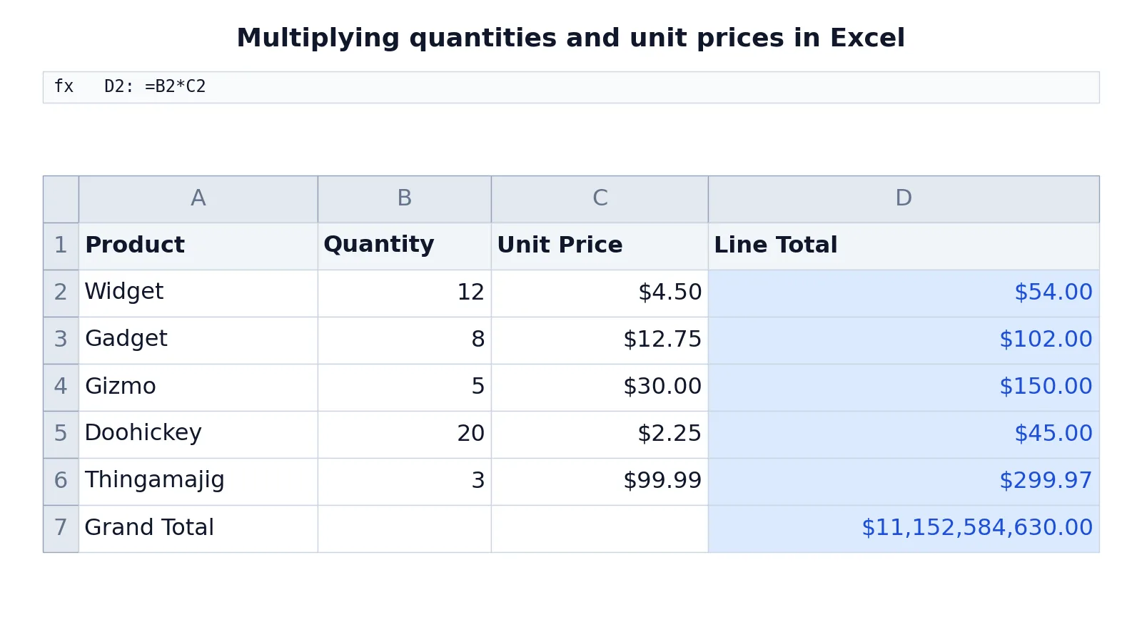
The table below is a small order sheet with a product name, a quantity, a unit price, and a line total for each row. The line totals multiply quantity by unit price, and the grand total multiplies every quantity by every unit price.

	A	B	C	D
1	Product	Quantity	Unit Price	Line Total
2	Widget	12	4.5	`=B2*C2` -> displays $54.00
3	Gadget	8	12.75	`=B3*C3` -> displays $102.00
4	Gizmo	5	30	`=B4*C4` -> displays $150.00
5	Doohickey	20	2.25	`=B5*C5` -> displays $45.00
6	Thingamajig	3	99.99	`=B6*C6` -> displays $299.97
7	Grand Total			`=PRODUCT(B2:B6,C2:C6)` -> displays $11,152,584,630.00

Row 2 multiplies 12 units by $4.50 to get $54.00. Rows 3 through 6 use the same pattern with their own values. The formula in D2 is filled down through D6, so each row multiplies its own quantity by its own unit price.

The grand total in D7 is the one to look at carefully. PRODUCT(B2:B6,C2:C6) multiplies all five quantities together and all five unit prices together, then multiplies those two results. That is not the sum of the line totals. It is a single product of ten numbers, which is why it lands in the billions. If you want the sum of the line totals, use =SUM(D2:D6) instead. The PRODUCT result is correct for what it computes, but it answers a different question than most people expect in a totals row.

How to Interpret the Result

A multiplication result is a product, and its meaning depends on the units of the inputs. Quantity times unit price gives a currency amount. A rate times a distance gives a distance. When both inputs are plain numbers, the product is a plain number.

Check the sign. Multiplying two positive numbers gives a positive result. Multiplying a positive by a negative gives a negative result. Multiplying two negatives gives a positive result. If a line total comes out negative, one of the inputs is negative, and that is usually a data entry problem rather than a math problem.

Check the magnitude. A product grows fast. Multiplying five numbers that are each around 10 gives a result in the hundreds of thousands, not the tens. When a total looks wildly larger than the individual rows, you probably used PRODUCT where SUM was intended.

Check the references. Click the result cell and look at the formula bar. If the formula points at the wrong cells, the number is wrong even though Excel did the arithmetic correctly.

Doing It in Software

In Excel, the asterisk operator and PRODUCT are the two tools for multiplication [1][2]. Both work in Excel for Microsoft 365, Excel 2024, Excel 2021, Excel 2019, and Excel 2016, on Windows and Mac [1].

A simple multiplication in a cell looks like this:

=B2*C2

A column multiplied by a fixed cell looks like this:

=B2*$B$10

A product across two ranges looks like this:

=PRODUCT(B2:B6,C2:C6)

If you work in Google Sheets, the same asterisk operator and the same PRODUCT function apply, and the steps are covered in How to Multiply in Google Sheets.

In R, multiplication uses the same asterisk:

quantity <- c(12, 8, 5, 20, 3)
price <- c(4.5, 12.75, 30, 2.25, 99.99)
line_total <- quantity * price
line_total

In Python with pandas, multiply two columns directly:

import pandas as pd
df = pd.DataFrame({"quantity": [12, 8, 5, 20, 3], "price": [4.5, 12.75, 30, 2.25, 99.99]})
df["line_total"] = df["quantity"] * df["price"]
print(df["line_total"])

For quick hand checks of fractions that involve multiplication, a Fraction Calculator handles the arithmetic without a spreadsheet.

Common Mistakes

Leaving out the asterisk. Writing =3(2+5) or =A1(A2) does not multiply in Excel. Add the between the operands, as in =3(2+5) [2].
Forgetting the equal sign. A cell entry that starts with a digit or letter is treated as text or a date, not a formula. Every formula begins with = [1].
Using a relative reference for a constant. If you drag =A2*B2 down a column, the reference shifts. Lock the constant cell with dollar signs, as in =A2*$B$2 [1].
Using PRODUCT for a totals row. PRODUCT multiplies everything you give it. A grand total of line items usually needs SUM, not PRODUCT.
Mixing text with numbers. A cell that holds non-numeric text produces a #VALUE! error with the * operator, and a number stored as text is ignored by PRODUCT when it sits in a range. Check the cell alignment, since text is left aligned by default and numbers are right aligned.
Pointing at the wrong range. Mixing up rows and columns in a range reference silently changes the result.

Limitations

Multiplication in Excel works on numbers only. Blank cells, text, and error values interfere with the result. PRODUCT ignores blank cells and text in a range, which can hide a missing value instead of flagging it. If a quantity cell is empty, the product simply skips it, and the total looks plausible while being wrong.

The asterisk operator has no built-in error handling. If one referenced cell contains an error, the whole formula returns that error. Multiplication also cannot tell you whether the inputs make sense. It will happily multiply a negative quantity by a price and return a negative total. Validation of the inputs is your job, not the formula's.

Frequently Asked Questions

What is the multiplication formula in Excel?

The multiplication formula in Excel uses the asterisk operator between two values or cell references, as in =A2*B2 [2]. You can also use the PRODUCT function to multiply several values or ranges at once. Both approaches start with an equal sign [1].

How do I multiply a whole column by one number in Excel?

Put the number in its own cell, then write the formula with an absolute reference to that cell, such as =A2*$B$2 [1]. The dollar signs keep the reference fixed when you drag the formula down the column. Without them, the reference shifts with each row [1].

What is the difference between the asterisk and PRODUCT in Excel?

The asterisk multiplies exactly the operands you list, so =A2*B2 multiplies two cells. PRODUCT multiplies every number in the arguments you give it, so =PRODUCT(B2:B6,C2:C6) multiplies ten values in one formula. Use the asterisk for simple pairs and PRODUCT for long lists or ranges.

Why does my multiplication formula return a #VALUE! error?

A #VALUE! error usually means one of the referenced cells contains text that Excel cannot read as a number, such as a word, a stray character, or a non-breaking space. Check each referenced cell and clean or convert those entries.

Can I multiply cells across different worksheets in Excel?

Yes. Reference the sheet name before the cell address, as in =Sheet2!A2*Sheet3!B2. The sheet name and the cell address are separated by an exclamation point. The same asterisk operator applies once the references are in place.

How do I multiply a range by a percentage in Excel?

Store the percentage in its own cell, then multiply with an absolute reference, as in =A2*$B$2. Format the percentage cell as a percentage so Excel stores it as a decimal. The result is the original value scaled by that percentage.

References

Further Reading
- Broman KW, Woo KH (2018). Data Organization in Spreadsheets. The American Statistician
- Ziemann M, Eren Y, El-Osta A (2016). Gene name errors are widespread in the scientific literature. Genome Biology
- Microsoft Support: Excel help and learning
- McCullough B, Heiser DA (2008). On the accuracy of statistical procedures in Microsoft Excel 2007. Computational Statistics & Data Analysis