How to Multiply in Google Sheets (Step by Step)
By Dr. Zubair Khalid, DVM, MS, PhD ·
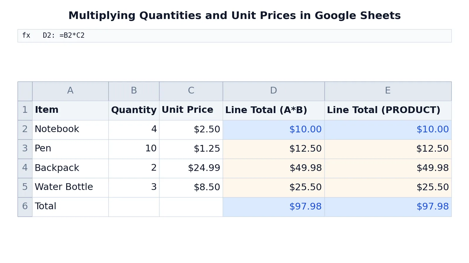
To multiply in Google Sheets, type an equals sign, then the first number or cell reference, then an asterisk (*), then the second number or cell reference. For example, =B2*C2 multiplies the values in those two cells. You can also use the PRODUCT function, as in =PRODUCT(B2:C2), which multiplies every number in a range.
Quick Answer
- The asterisk
*is the multiplication operator in Google Sheets. Write=A1*B1to multiply two cells. - The PRODUCT function multiplies a list or range:
=PRODUCT(A1:B1)or=PRODUCT(A1,B1,C1). - Both methods return the same result for the same inputs.
- Multiplication has higher precedence than addition and subtraction, so
=2+3*4returns 14, not 20. - Use parentheses to control order, since brackets change how a formula is evaluated [1].
Before You Start
You need a Google account and a spreadsheet open in Google Sheets. No add-ons or special settings are required for basic multiplication.
Two things help before you write formulas. First, decide whether your numbers are typed directly into the formula or stored in cells. Cell references are almost always better because you can change a value and the result updates automatically. Second, check that your numbers are real numbers and not text. A number stored as text looks fine on screen but breaks multiplication.
If you are new to writing formulas at all, the structure is the same across spreadsheet tools, and the basics of building one are covered in this guide to making a formula in Excel, which transfers directly to Google Sheets.
Step by Step
- Click the cell where you want the result. For a line total, that is the first empty cell in the total column.
- Type
=to start the formula. - Type the first cell reference, for example
B2. - Type
*for multiplication. - Type the second cell reference, for example
C2. - Press Enter. The cell shows the product.
So the full formula is =B2*C2. Google Sheets reads it as "take the value in B2 and multiply it by the value in C2."
To multiply more than two cells, keep adding * and references: =B2*C2*D2. To multiply a whole range in one go, switch to PRODUCT: =PRODUCT(B2:C2).
If you want to multiply a column of values by a single number, put that number in one cell and reference it with absolute references, for example =A2*$F$1. The dollar signs lock the reference so it does not shift when you copy the formula down.
Worked Example
This example is a small order sheet with four items. Columns B and C hold quantity and unit price, and columns D and E compute line totals two different ways so you can compare them.
| Row | A | B | C | D | E |
|---|---|---|---|---|---|
| 1 | Item | Quantity | Unit Price | Line Total (A*B) | Line Total (PRODUCT) |
| 2 | Notebook | 4 | 2.5 | =B2*C2 -> displays $10.00 | =PRODUCT(B2:C2) -> displays $10.00 |
| 3 | Pen | 10 | 1.25 | =B3*C3 -> displays $12.50 | =PRODUCT(B3:C3) -> displays $12.50 |
| 4 | Backpack | 2 | 24.99 | =B4*C4 -> displays $49.98 | =PRODUCT(B4:C4) -> displays $49.98 |
| 5 | Water Bottle | 3 | 8.5 | =B5*C5 -> displays $25.50 | =PRODUCT(B5:C5) -> displays $25.50 |
| 6 | Total | =SUM(D2:D5) -> displays $97.98 | =SUM(E2:E5) -> displays $97.98 |
The first line total uses the asterisk operator. In D2, =B2*C2 multiplies 4 by 2.5 and returns $10.00. The second column does the same job with the function. In E2, =PRODUCT(B2:C2) multiplies every number in the range B2 through C2 and also returns $10.00.
Both columns agree on every row. The order total in D6 sums the asterisk results with =SUM(D2:D5) and returns $97.98. The total in E6 sums the PRODUCT results with =SUM(E2:E5) and returns the same $97.98.
The takeaway is that the operator and the function are interchangeable for two cells. PRODUCT becomes more convenient when you multiply three or more values, because you write one range instead of a chain of asterisks. Summing the results afterward is the same operation you would use to add up any column, and the mechanics are covered in this guide to summing a column in Excel.
Other Ways to Do It
The PRODUCT function with a range. =PRODUCT(B2:C2) multiplies all numbers in the range. This is the cleanest option for three or more factors.
The PRODUCT function with separate arguments. =PRODUCT(B2,C2,D2) multiplies individual cells or values. You can mix references and typed numbers, as in =PRODUCT(B2,2,3).
Multiplying by a constant. =B2*1.08 multiplies a cell by a fixed number, useful for applying a rate or markup.
Array-style multiplication. In Google Sheets you can multiply two ranges element by element with =ARRAYFORMULA(A2:A10*B2:B10), which returns one product per row. This is a Sheets-specific convenience and behaves differently from Excel, where you would enter a similar formula differently.
Copying a formula down. After you write =B2*C2 in D2, you can drag the fill handle down the column. Relative references adjust row by row, so D3 becomes =B3*C3 automatically.
Troubleshooting
The result is a #VALUE! error. One of the cells contains text that cannot be converted to a number. Check for stray spaces, apostrophes, or labels in the referenced cells.
The result is 0. A referenced cell is empty or holds a zero. Empty cells are treated as zero in multiplication, so the whole product collapses to zero.
The formula shows as text. The cell is formatted as plain text, or the formula is missing the leading =. Reformat the cell as a number and retype the formula.
The result is wrong but not an error. Check operator precedence. =2+3*4 returns 14 because multiplication runs before addition. Add parentheses to change the order, since brackets control how a formula is evaluated [1].
The formula breaks when copied. You likely need absolute references. Use $ signs, as in $F$1, to lock a cell that should not shift.
Common Mistakes
- Forgetting the equals sign. Typing
B2*C2without=leaves the text in the cell. Start every formula with=. - Using the letter x instead of the asterisk.
=B2xC2is not valid. The multiplication operator is*. - Ignoring operator precedence.
=A1+B1*C1multiplies first, then adds. Wrap the addition in parentheses if you want it done first [1]. - Referencing text cells. A number stored as text returns
#VALUE!. Convert it to a real number before multiplying. - Mixing up relative and absolute references. Copying
=A2*F1down shifts both references. Lock the constant with$F$1. - Multiplying when you meant to sum. PRODUCT multiplies. If you want a total of values, use SUM instead.
Limitations
Multiplication in Google Sheets is exact for ordinary decimal arithmetic, but floating-point storage means some decimal results carry tiny rounding differences. Values like 0.1 and 0.2 do not always add or multiply to a clean decimal, so a displayed $49.98 may sit on a value like 49.980000000000004 internally. For money, format the cell to two decimals so the display matches what you expect.
PRODUCT ignores empty cells and text, which is convenient but can hide data problems. If a cell you expected to contain a number is actually blank, PRODUCT silently skips it and returns a product of the remaining values instead of an error. The asterisk operator behaves differently, treating an empty cell as zero and returning zero. That difference matters when you audit a sheet, so pick one method and apply it consistently across a column.
Frequently Asked Questions
How do I multiply a whole column in Google Sheets?
Write the formula in the first cell, for example =B2*C2, then drag the fill handle down the column. Each row adjusts automatically because the references are relative. For a single formula that fills the column at once, use =ARRAYFORMULA(B2:B10*C2:C10).
What is the difference between * and PRODUCT in Google Sheets?
Both multiply values and return the same result for the same inputs. The asterisk operator multiplies two values at a time and treats empty cells as zero. PRODUCT accepts a range or a list and skips empty cells and text. Use * for simple pairs and PRODUCT for longer lists or ranges.
How do I multiply two columns and then add the results?
Multiply each row in its own cell, then sum the column. In the worked example, =B2*C2 fills column D and =SUM(D2:D5) returns $97.98. You can also combine both steps in one formula with =SUMPRODUCT(B2:B5,C2:C5), which multiplies each pair and adds the products.
Why does my multiplication formula return 0?
At least one referenced cell is empty or contains zero. Google Sheets treats an empty cell as zero in multiplication, so the product becomes zero. Fill the missing value or check that the reference points to the right cell.
Can I multiply numbers in different sheets?
Yes. Reference the other sheet by name, as in =Sheet2!B2*C2. If the sheet name contains spaces, wrap it in single quotes, as in ='Unit Prices'!B2*C2. The multiplication itself works the same way.
References
Further Reading
- Broman KW, Woo KH (2018). Data Organization in Spreadsheets. The American Statistician
- Ziemann M, Eren Y, El-Osta A (2016). Gene name errors are widespread in the scientific literature. Genome Biology
- Microsoft Support: Excel help and learning
- McCullough B, Heiser DA (2008). On the accuracy of statistical procedures in Microsoft Excel 2007. Computational Statistics & Data Analysis
- Abeysooriya M, Soria M, Kasu MS et al. (2021). Gene name errors: Lessons not learned. PLOS Computational Biology