Quantitative Data Examples: Definition and Types

By Dr. Zubair Khalid, DVM, MS, PhD · 2026-10-03

Quantitative data examples are everywhere in research and everyday life: a person's age, a package's weight, a test score, a monthly rent payment. Each of these is a number produced by counting or measuring something. The key distinction is whether the number comes from counting (discrete) or measuring (continuous), and that difference shapes how you summarize and graph the data.

Quick Answer

Quantitative data are always numbers, and they result from counting or measuring attributes of a population [1].
Discrete data come from counting and take only certain numerical values, such as the number of phone calls you receive in a day [1].
Continuous data come from measuring and can include fractions, decimals, or irrational numbers, such as lengths, weights, or times [1].
Common quantitative data examples include height, number of exams, temperature, salary, volume, and speed [2].
Both types can be summarized with a mean, median, and range, but continuous values usually need rounding rules and wider class intervals when you build a frequency table [3].

What Quantitative Data Means

In plain terms, quantitative data is information you can express as a number and compare mathematically. If you can add it, average it, or rank it on a number line, it is quantitative.

The precise statistical definition is narrower. Quantitative data are the result of counting or measuring attributes of a population, and they may be either discrete or continuous [1]. Amount of money, pulse rate, weight, the number of people living in your town, and the number of students who take statistics are all examples of quantitative data [1]. This separates it from qualitative data, which deals with descriptions and qualities that are observed instead of measured by numbers, such as political affiliation, colors, or feelings about a topic [2].

Quantitative research investigates phenomena that can be quantified with numbers or statistics resulting from formal measurement, and it typically involves experimentation, surveys, or questionnaires in the context of a large, randomly selected group [4]. That is why quantitative studies tend to report their findings in tables, charts, and graphs [4].

How It Works

The mechanism behind quantitative data is simple: you either count or you measure, and the method you used determines the type.

Discrete data come from counting. These data take on only certain numerical values [1]. If you count the number of phone calls you receive each day of the week, you might get values such as zero, one, two, or three [1]. You cannot receive 2.4 phone calls. The values are whole numbers with gaps between them.

Continuous data come from measuring. Data that are not only made up of counting numbers, but that may include fractions, decimals, or irrational numbers, are called quantitative continuous data [1]. Continuous data are often the results of measurements like lengths, weights, or times [1]. A list of the lengths in minutes for all the phone calls you make in a week, with numbers like 2.4, 7.5, or 11.0, would be quantitative continuous data [1].

Once you have the numbers, you summarize them with descriptive statistics. The three most common are:

$$\bar{x} = \frac{\sum_{i=1}^{n} x_i}{n}$$

Here $\bar{x}$ is the mean, $\sum x_i$ is the sum of all values, and $n$ is the number of values. The median is the middle value when the data are sorted, or the average of the two middle values when $n$ is even. The range is:

$$\text{Range} = \max(x) - \min(x)$$

where $\max(x)$ is the largest value and $\min(x)$ is the smallest.

Worked Example

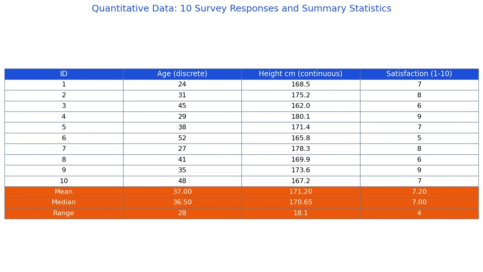
This example uses a survey of 10 respondents with age (discrete), height in centimeters (continuous), and a satisfaction score from 1 to 10.

respondent_id	age_years	height_cm	satisfaction_1_10
1	24	168.5	7
2	31	175.2	8
3	45	162.0	6
4	29	180.1	9
5	38	171.4	7
6	52	165.8	5
7	27	178.3	8
8	41	169.9	6
9	35	173.6	9
10	48	167.2	7

Age (discrete). With $n = 10$, the mean is $(24+31+45+29+38+52+27+41+35+48) / 10 = 37.0000$. Sorted, the values are [24, 27, 29, 31, 35, 38, 41, 45, 48, 52]. The middle two are 35 and 38, so the median is $(35+38)/2 = 36.5000$. The range is $52 - 24 = 28$.

Height (continuous). With $n = 10$, the sum is 1712.0, so the mean is $1712.0 / 10 = 171.2000$. Sorted, the values are [162.0, 165.8, 167.2, 168.5, 169.9, 171.4, 173.6, 175.2, 178.3, 180.1]. The middle two are 169.9 and 171.4, so the median is $(169.9+171.4)/2 = 170.6500$. The range is $180.1 - 162.0 = 18.1000$.

Satisfaction (discrete, bounded). With $n = 10$, the mean is $(7+8+6+9+7+5+8+6+9+7) / 10 = 7.2000$. Sorted, the values are [5, 6, 6, 7, 7, 7, 8, 8, 9, 9]. The middle two are both 7, so the median is $(7+7)/2 = 7.0000$. The range is $9 - 5 = 4$.

Here is the same computation in Python:

import statistics
ages = [24, 31, 45, 29, 38, 52, 27, 41, 35, 48]
heights = [168.5, 175.2, 162.0, 180.1, 171.4, 165.8, 178.3, 169.9, 173.6, 167.2]
sats = [7, 8, 6, 9, 7, 5, 8, 6, 9, 7]
for name, x in [('age', ages), ('height', heights), ('satisfaction', sats)]:
    print(name, f"{statistics.fmean(x):.4f}", f"{statistics.median(x):.4f}", round(max(x)-min(x), 4))

Output:

age 37.0000 36.5000 28
height 171.2000 170.6500 18.1
satisfaction 7.2000 7.0000 4

How to Interpret It

Read the mean and median together. For age, the mean is 37.0000 and the median is 36.5000, so the two are close and the distribution is roughly balanced. For height, the mean is 171.2000 and the median is 170.6500, again close, which suggests no strong skew.

The range tells you the spread. Age spans 28 years, which is wide for 10 people. Height spans 18.1 cm. Satisfaction spans only 4 points, which is narrow because the scale itself is bounded from 1 to 10.

The type of data changes how you present it. The graph of a frequency distribution for quantitative data is called a frequency histogram, or histogram for short [3]. When you group continuous values into classes, the class width should be rounded up to the nearest value with the same number of decimal places as the original data, and the class boundaries should have one more decimal place than the original data [3]. For example, if your data has one decimal place, the class width would have one decimal place, and the class boundaries are formed by adding and subtracting 0.05 from each class limit [3]. Pie charts are possible for quantitative data, but their usefulness varies with the number of intervals, and a pie chart of weight data is difficult to read because of the quantity of intervals used [6].

When to Use It (and when not to)

Use quantitative data when your question is about amount, frequency, or magnitude. If you want to know how many, how much, how often, or how long, you need numbers. Quantitative research is the right frame when you are comparing two variables using numerical data [4]. Heart rates, blood cell counts, and how many people fainted at an event are all examples of quantitative measures [5].

Do not force quantitative data where the underlying concept is descriptive. Gender, country name, animal species, and emotional state are examples of qualitative information [7]. You can code them as numbers, but the numbers carry no arithmetic meaning. Averaging zip codes or jersey numbers produces nonsense.

Also avoid treating a bounded discrete score as continuous. A satisfaction score of 7.2 is a mean, not an observation. No single respondent gave 7.2.

Quantitative vs Qualitative Data

Feature	Quantitative	Qualitative
Core content	Numbers from counting or measuring [1]	Descriptive judgments using concept words [7]
Examples	Height, number of exams, temperature, salary, volume, speed [2]	Political affiliation, colors, feelings, open-ended exam responses [2]
Objectivity	Tends to be more objective and finite [7]	Can be objective or subjective [7]
Typical presentation	Tables, charts, graphs, histograms [4]	Interview transcripts, focus group feedback, journal entries [5]
Subtypes	Discrete and continuous [1]	Nominal and ordinal categories

If you want a deeper side-by-side treatment, see Qualitative vs Quantitative Data: Types and Examples.

Common Mistakes

Calling any number quantitative. A number used as a label, such as a student ID, is not quantitative. Fix: ask whether arithmetic on the value is meaningful.
Treating discrete counts as continuous. You cannot have 2.4 phone calls. Fix: keep counts as whole numbers and round only summary statistics.
Treating continuous measurements as discrete. Height of 168.5 cm is a real measurement, not a rounding error. Fix: keep the decimal places your instrument reports.
Averaging ordinal or coded categories. Satisfaction scores are bounded and ordered, so a mean is a rough summary at best. Fix: report the median and the full distribution alongside the mean.
Ignoring class width rules for continuous data. Class boundaries need one more decimal place than the original data [3]. Fix: set boundaries by adding and subtracting 0.05 when your data has one decimal place.
Reporting a mean with no spread. A mean alone hides variability. Fix: always pair it with the range, standard deviation, or an interquartile range.

Limitations

Quantitative data cannot capture meaning, context, or motivation. A satisfaction score of 5 tells you where someone landed on a scale, but not why. Numbers also depend entirely on how the variable was defined and measured, so two studies can report the same variable with different values because their instruments or definitions differ.

Summary statistics compress information and can mislead. A mean can sit where no individual value exists, and a range is sensitive to a single extreme observation. With small samples, such as the 10 respondents above, the mean and median can shift noticeably when one value changes. Quantitative analysis also assumes the measurement scale behaves as expected, which is a weak assumption for bounded rating scales.

Frequently Asked Questions

What are some examples of quantitative data?

Age, height, weight, temperature, salary, pulse rate, number of books in a backpack, number of machines in a gym, and phone call duration are all quantitative data [1]. Each is a number produced by counting or measuring. They split into discrete types, like counts, and continuous types, like measurements.

What is the difference between discrete and continuous data?

Discrete data come from counting and take on only certain numerical values, such as zero, one, two, or three phone calls in a day [1]. Continuous data come from measuring and may include fractions, decimals, or irrational numbers, such as lengths, weights, or times [1]. The practical test is whether a value between two others is possible.

Is age discrete or continuous?

Age in whole years is discrete because you count completed years. Age measured precisely, such as 24.37 years, is continuous because it comes from measurement on a fine scale. The type depends on how you recorded it, not on the concept itself.

Can quantitative data be non-numeric?

No. Quantitative data are always numbers [1]. If your data consist of words, images, or descriptions, they are qualitative. You can convert qualitative categories into numeric codes, but the codes are labels, not measurements.

How do I summarize quantitative data?

Start with the mean, median, and range, then add a histogram to show the shape of the distribution [3]. For grouped continuous data, choose class intervals and follow the decimal-place rules for class width and boundaries [3]. If you are working with a full table of variables, see What Is a Dataset? Definition, Types and Examples for how to organize the columns before you summarize.

References

1.2: Data, Sampling, and Variation in Data and Sampling - Statistics LibreTexts/01%3A_Sampling_and_Data/1.02%3A_Data_Sampling_and_Variation_in_Data_and_Sampling)
Definitions and Examples | Data Visualization Award
2.2: Quantitative Data - Statistics LibreTexts
Quantitative Research - Quantitative and Qualitative Research - Seton Hall University Libraries at Seton Hall University
Qualitative vs. Quantitative Research - Nursing Research Guide - Research Guides at Texas A&M University-Corpus Christi
8.2: Presenting Quantitative Data Graphically - Statistics LibreTexts/08%3A_Describing_Data/8.02%3A_Presenting_Quantitative_Data_Graphically)
Qualitative vs. Quantitative Research - CJS 315: Research Methods in Crime and Justice Studies - Research Guides at University of Massachusetts Dartmo