How to Calculate Variance: Formula, Steps and Examples
By Dr. Zubair Khalid, DVM, MS, PhD ·
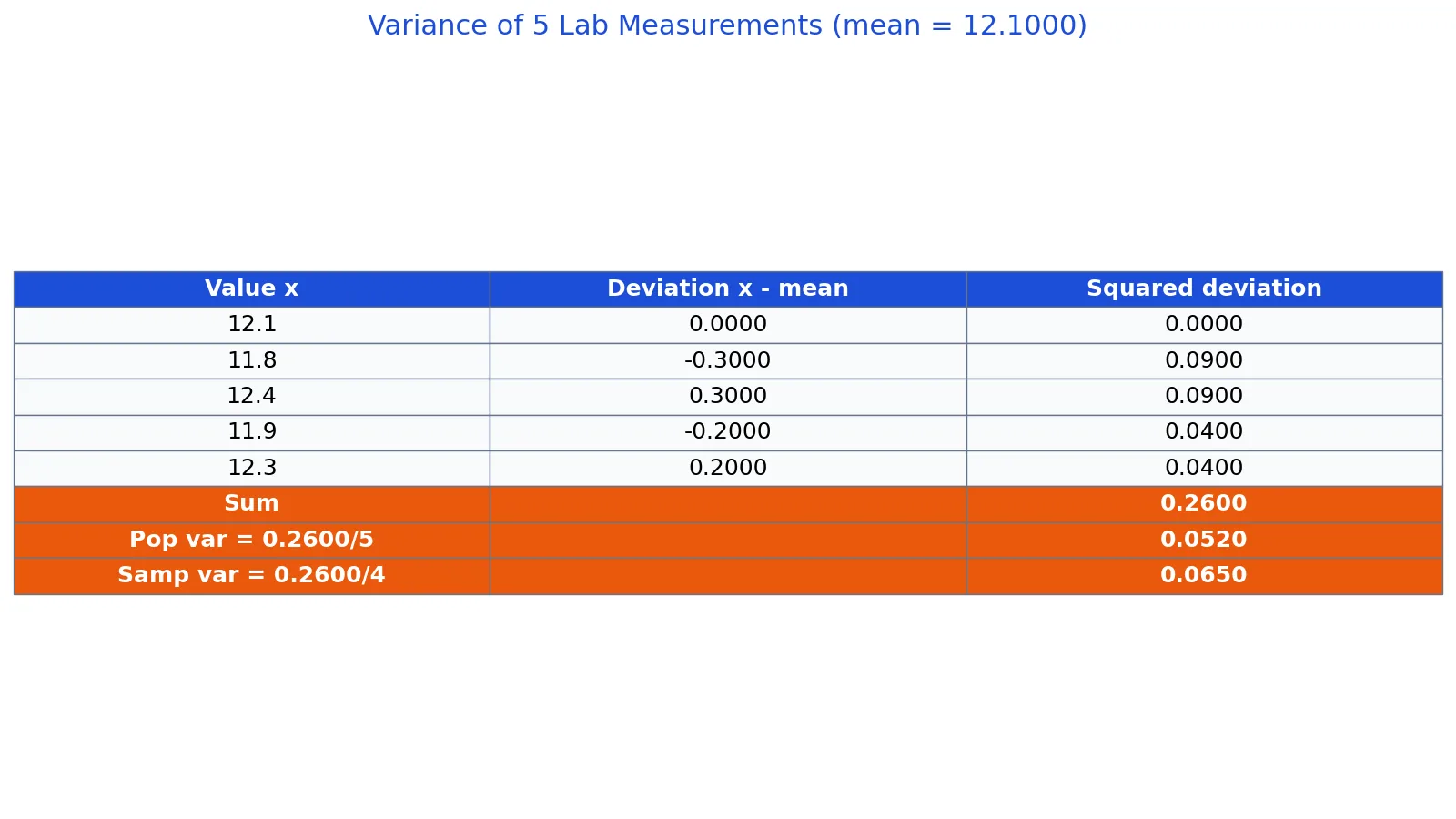
To calculate variance, subtract the mean from each value, square each deviation, add the squared deviations, then divide by N for a population or n - 1 for a sample. The result tells you how spread out the data is around the mean. This guide shows how to calculate variance by hand, with a calculator, and in code, using one dataset throughout.
Quick Answer
- Variance measures the average squared distance of each value from the mean.
- Population variance: $\sigma^2 = \frac{\sum (x_i - \mu)^2}{N}$, divide by the number of values.
- Sample variance: $s^2 = \frac{\sum (x_i - \bar{x})^2}{n - 1}$, divide by one less than the number of values.
- The numerator, the sum of squared deviations, is the same for both. Only the denominator changes.
- Variance is in squared units, so take the square root to get the standard deviation.
What Is Variance and How Do You Calculate It?
To calculate variance, find the mean, subtract it from every value, square each result, add the squares, then divide by N for a population or n - 1 for a sample. The answer is a single number that describes how spread out the values are around the mean. A small variance means the values sit close to the mean; a large variance means they scatter widely.
The formula in words: variance equals the sum of squared deviations divided by the count. In symbols, population variance is $\sigma^2 = \frac{\sum (x_i - \mu)^2}{N}$ and sample variance is $s^2 = \frac{\sum (x_i - \bar{x})^2}{n - 1}$. The top part of the fraction, the sum of squared deviations, is identical in both. Only the bottom changes.
Sample variance is the version you use most often, because real datasets are usually subsets of a larger group. Dividing by n - 1 instead of n corrects a built-in downward bias, so the sample result estimates the wider population more fairly. With five values, that means dividing by 4, not 5.
Comparing two numbers is a different job from measuring spread. If you have just two values, say 40 and 60, the variance formula still works: the mean is 50, each deviation is 10, the squares are 100 and 100, the sum is 200, and dividing by 2 gives a population variance of 100 (or by 1 for a sample variance of 200). But with only two points you learn almost nothing about spread, so people usually want the gap or the percent change instead.
| What you have | What to compute | Quick method |
|---|---|---|
| Two raw values | Difference | Subtract the smaller from the larger |
| Two raw values | Percent difference | Divide the difference by the average of the two, times 100 |
| An old value and a new value | Percent change | Divide the change by the starting value, times 100 |
| A full column of values | Variance | Mean, deviations, squares, divide by N or n - 1 |
For a percentage version of variance, statisticians use the coefficient of variation: the standard deviation divided by the mean, times 100. That expresses spread as a percent of the average, which lets you compare datasets measured in different units.
Before You Start
You need one column of numeric values and a decision about whether it is a sample or a population. A population is every member of the group you care about. A sample is a subset drawn from a larger group. In practice, most datasets are samples, so you divide by n - 1.
You also need the mean first, because every deviation is measured from it. If you want a refresher, see how to calculate the mean before continuing.
Two formulas describe the same idea. The definitional formula uses deviations from the mean, which is what this article walks through. The computational formula uses raw sums of squares and is faster on a calculator, but it is more prone to rounding error. The NIST handbook shows both styles in its ANOVA calculations, where sums of squares are built from raw values and then corrected for the mean [1].
Step by Step
- Count your values. Call the count N for a population or n for a sample.
- Find the mean. Add every value and divide by the count.
- Subtract the mean from each value. These are the deviations. They always sum to zero, which is a useful check.
- Square each deviation. Squaring removes the sign and makes large gaps count more.
- Add the squared deviations. This total is the sum of squares.
- Divide. Use N for population variance or n - 1 for sample variance.
In symbols, the population formula is:
$$\sigma^2 = \frac{\sum_{i=1}^{N}(x_i - \mu)^2}{N}$$
The sample formula is:
$$s^2 = \frac{\sum_{i=1}^{n}(x_i - \bar{x})^2}{n - 1}$$
The n - 1 denominator is called Bessel's correction. Dividing by n - 1 makes the sample variance an unbiased estimate of the population variance, because a sample tends to be less spread out than the population it came from.
Worked Example
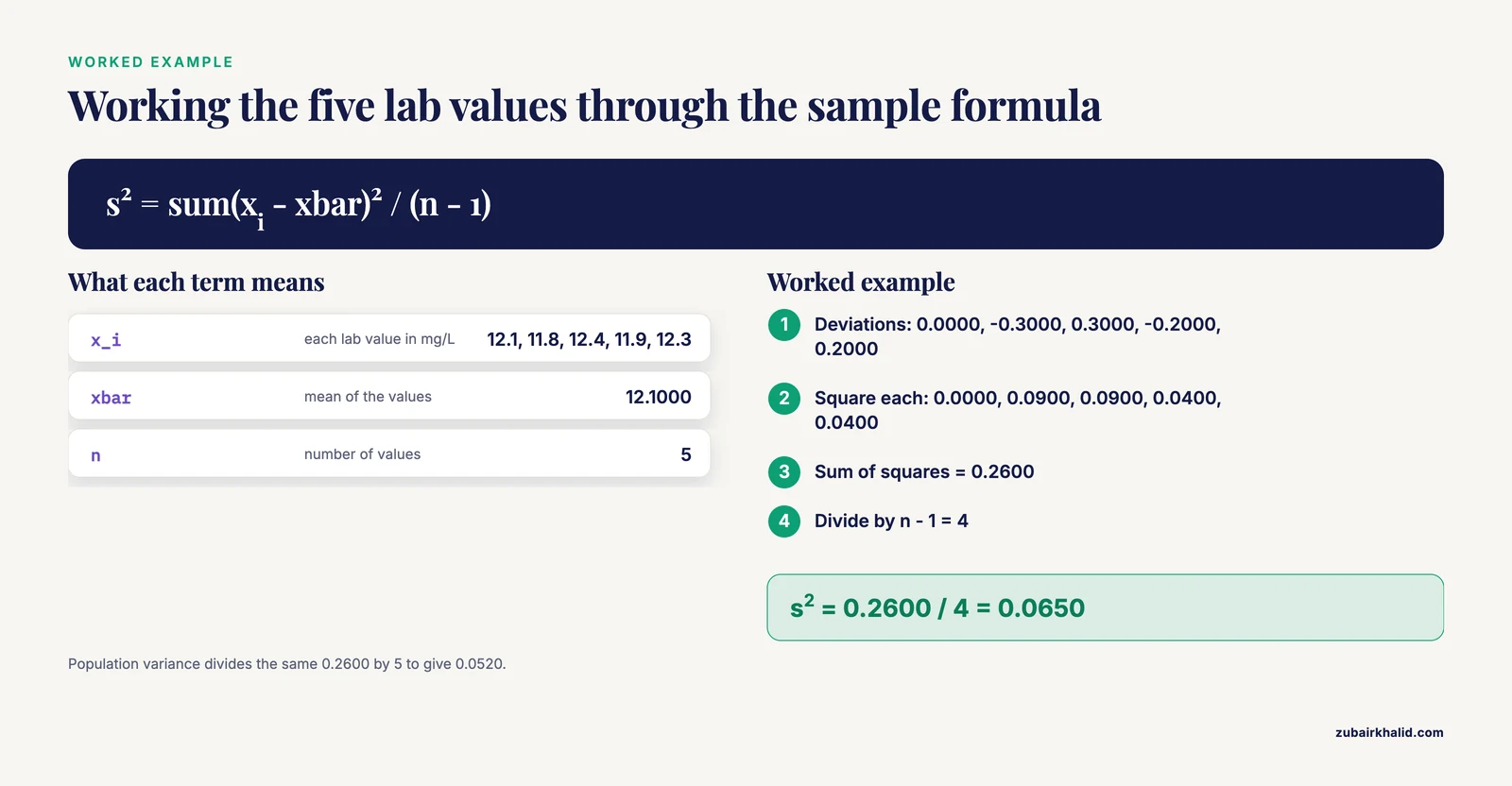
Five lab measurements of a sample concentration, in mg/L, are 12.1, 11.8, 12.4, 11.9, and 12.3.
| Value | Deviation from mean (12.1000) | Squared deviation |
|---|---|---|
| 12.1 | 0.0000 | 0.0000 |
| 11.8 | -0.3000 | 0.0900 |
| 12.4 | 0.3000 | 0.0900 |
| 11.9 | -0.2000 | 0.0400 |
| 12.3 | 0.2000 | 0.0400 |
The mean is (12.1 + 11.8 + 12.4 + 11.9 + 12.3) / 5 = 12.1000.
The squared deviations add to 0.0000 + 0.0900 + 0.0900 + 0.0400 + 0.0400 = 0.2600.
Population variance: 0.2600 / 5 = 0.0520.
Sample variance: 0.2600 / 4 = 0.0650.
The population standard deviation is sqrt(0.0520) = 0.2280, and the sample standard deviation is sqrt(0.0650) = 0.2550. Notice how the deviations cancel to zero before squaring, which confirms the mean was correct.
Here is the same calculation in Python:
import numpy as np
data = [12.1, 11.8, 12.4, 11.9, 12.3]
print(f"numpy ddof=0 = {np.var(data, ddof=0):.4f}")  # population variance
print(f"numpy ddof=1 = {np.var(data, ddof=1):.4f}")  # sample variance
Output:
numpy ddof=0 = 0.0520
numpy ddof=1 = 0.0650The ddof argument sets the delta degrees of freedom. ddof=0 divides by N, and ddof=1 divides by n - 1.
Other Ways to Do It
Spreadsheet. In Excel, VAR.P returns population variance and VAR.S returns sample variance. The full walkthrough is in how to calculate variance in Excel.
Calculator. Many scientific and graphing calculators have a statistics mode that reports both values. You enter the data list, run the one-variable statistics command, and read the population and sample results. The labels differ by model, so check which symbol the display uses before you record the answer. If you want to skip the manual entry, the variance calculator returns both figures from a pasted list.
By hand with the computational formula. Square every value, add them, subtract the correction term $(\sum x)^2 / n$, then divide. This avoids computing each deviation separately but loses precision when values are large.
Troubleshooting
If your deviations do not sum to zero, the mean is wrong. Recheck the addition.
If the variance is negative, you made an arithmetic error. Squared numbers cannot be negative, so the sum of squares is always zero or positive.
If the sample and population answers look far apart, the sample is small. With n = 5, dividing by 4 instead of 5 raises the result by 25 percent. The gap shrinks as n grows.
If a calculator gives a different answer, check whether it is reporting the standard deviation instead of the variance. The standard deviation is the square root of the variance, so it is always smaller for values above 1.
If your data has units, the variance carries squared units. A variance of 0.0520 in mg/L data is in mg²/L², which is why analysts usually report the standard deviation instead.
Common Mistakes
- Dividing by n when you have a sample. Use n - 1 for sample variance. Dividing by n underestimates the spread of the wider population.
- Forgetting to square before adding. Adding raw deviations gives zero every time. Square first, then sum.
- Squaring after summing. The order matters. Each deviation is squared individually, then the squares are added.
- Rounding the mean too early. Keep at least four decimal places in the mean, or the squared deviations drift. In the example, the mean is exactly 12.1000, but that is not typical.
- Confusing variance with standard deviation. Variance is in squared units. If you need the original units, take the square root. See how to calculate standard deviation.
- Mixing up the two symbols. $\sigma^2$ is the population variance and $s^2$ is the sample variance. Using the wrong one changes the reported result.
Limitations
Variance is sensitive to outliers because deviations are squared. One extreme value can dominate the sum of squares and make the spread look much larger than it is. If your data has heavy tails or extreme values, report the median and interquartile range alongside the variance.
Variance also assumes the values are measured on an interval or ratio scale. It is meaningless for categorical data, and it says nothing about the shape of the distribution. Two datasets can share a variance while looking completely different. The equal-variance assumption matters in tests like ANOVA, where the pooled variance is used and unequal group variances can distort the result [2]. When group sizes are roughly equal, the F-test stays valid if the largest variance is no more than four times the smallest [2].
Variance Between Two Numbers: What People Usually Mean
When someone asks for the variance between two numbers, they almost never want the statistical variance. They want the gap or the percent difference. Here is how to tell which one you need and how to compute each.
The plain difference
Take the larger value minus the smaller value. If a reading goes from 12.1 to 12.4 mg/L, the difference is 0.3 mg/L. This is the simplest measure and keeps the original units. It tells you the size of the gap but not how big that gap is relative to the values themselves.
Percent difference between two values
Percent difference compares two values without treating either as a starting point. Add the two values, divide by 2 to get their average, then divide the gap by that average and multiply by 100.
Worked example: compare 40 and 60.
- Gap: 60 - 40 = 20
- Average: (40 + 60) / 2 = 50
- Percent difference: (20 / 50) x 100 = 40 percent
So the two numbers differ by 40 percent of their average. This measure is symmetric: swapping 40 and 60 gives the same answer.
Percent change from an old value to a new value
Percent change treats one value as the starting point. Subtract the old value from the new value, divide by the old value, then multiply by 100.
Worked example: a price rises from 80 to 100.
- Change: 100 - 80 = 20
- Percent change: (20 / 80) x 100 = 25 percent increase
Reverse it: from 100 down to 80 is (80 - 100) / 100 x 100 = -20 percent, a 20 percent decrease. Notice that a 25 percent rise and a 20 percent fall do not cancel, because they are measured against different starting points. This is one of the most common sources of confusion in everyday percentage work.
When the statistical variance of two numbers is the right tool
Use the variance formula on two values only when you are treating them as a tiny dataset and you genuinely want a spread measure, for example as a stepping stone in a larger calculation. Otherwise, report the difference or the percent difference, which are easier to interpret and keep meaningful units.
Percentage Variance and the Coefficient of Variation
Variance itself is in squared units, so it cannot be written as a percent. What people call percentage variance is usually one of two things: the coefficient of variation, or a percent difference between two summary numbers.
The coefficient of variation
The coefficient of variation (CV) is the standard deviation divided by the mean, multiplied by 100. It converts spread into a percentage of the average, which makes datasets with different units or very different means comparable.
Worked example using the article's five concentrations (12.1, 11.8, 12.4, 11.9, 12.3 mg/L):
- Mean: 12.1000
- Sample standard deviation: 0.2550
- CV: (0.2550 / 12.1000) x 100 = about 2.11 percent
Interpretation: the typical distance from the mean is roughly 2 percent of the mean itself. A CV of 2 percent suggests tight, consistent measurements. A CV of 30 percent in the same kind of assay would suggest a process that needs attention. Because CV has no units, you can compare a set of mg/L readings with a set of gram readings directly.
One caution: the CV is unstable when the mean is near zero, because dividing by a tiny number produces a huge percentage. It also assumes the data are measured on a ratio scale with a true zero, so it is not appropriate for temperatures in Celsius or Fahrenheit.
Percent variance between two summary values
In quality control and finance, people sometimes say "variance" when they mean the percent gap between a target and an actual figure. The calculation is the same as percent change: (actual - target) / target x 100. If a batch target is 500 units and the actual is 460, the shortfall is (460 - 500) / 500 x 100 = -8 percent. This is a business comparison, not a statistical variance, and the two should not be mixed in the same report without a label.
A comparison table
| Measure | Formula | Units | Best used for |
|---|---|---|---|
| Variance | Sum of squared deviations / N or n - 1 | Squared units | Describing spread within one dataset |
| Standard deviation | Square root of variance | Original units | Reporting spread in readable units |
| Coefficient of variation | (Standard deviation / mean) x 100 | Percent | Comparing spread across datasets |
| Percent difference | Gap / average x 100 | Percent | Comparing two values with no baseline |
| Percent change | (New - old) / old x 100 | Percent | Tracking one value over time |
Checking Your Work: A Second Full Example
The article's five-value example has a mean that lands exactly on a data point, which hides rounding problems. Here is a messier dataset so you can see the arithmetic under realistic conditions.
Data: 4, 8, 15, 16, 23, 42. This is six values, so n = 6.
Step 1: the mean. Sum: 4 + 8 + 15 + 16 + 23 + 42 = 108. Mean: 108 / 6 = 18.
Step 2: deviations and squares.
| Value | Deviation from 18 | Squared deviation |
|---|---|---|
| 4 | -14 | 196 |
| 8 | -10 | 100 |
| 15 | -3 | 9 |
| 16 | -2 | 4 |
| 23 | 5 | 25 |
| 42 | 24 | 576 |
Step 3: check the deviations. -14 - 10 - 3 - 2 + 5 + 24 = 0. The mean is correct.
Step 4: sum of squares. 196 + 100 + 9 + 4 + 25 + 576 = 910.
Step 5: divide. Population variance: 910 / 6 = 151.67 (rounded). Sample variance: 910 / 5 = 182.00.
Step 6: standard deviations. Population: sqrt(151.67) = 12.32. Sample: sqrt(182.00) = 13.49.
Notice how the single value 42 contributes 576 out of 910, more than half the total sum of squares. That is the outlier sensitivity described in the article's limitations section in action. Remove 42 and the sample variance of the remaining five values drops to 35.70, a dramatic change from 182.00. This is why analysts look at the data before trusting a variance figure.
A visual way to think about it
Picture a number line with the mean marked as a peg. Each data point is a bead on the line. The deviation is the distance from the peg to the bead. Squaring turns each distance into an area of a square whose side is that distance. The variance is the average area of those squares. A far-out bead like 42 creates a huge square that dominates the average, which is exactly why one extreme value can inflate the variance so much.
Common misconceptions about this example
- "The variance should be between the smallest and largest values." It often is not. Here the sample variance of 182.00 is far above the largest value of 42, because squaring pushes large deviations up fast.
- "Dividing by 6 and by 5 should give nearly the same answer." With small n they differ by 20 percent here (151.67 versus 182.00). The gap only becomes negligible when n is large.
- "The mean of 18 is a typical value." It sits in a gap between 16 and 23. A mean is a balance point, not necessarily a common value, and variance says nothing about where the data cluster.
Reading Variance Correctly and Avoiding Traps
Squared units and why standard deviation is usually reported
A variance of 182.00 for data measured in grams is in grams squared, a unit with no physical meaning. Taking the square root returns 13.49 grams, which you can compare directly with the data. Report the standard deviation for communication and keep the variance for calculations such as ANOVA, where variances are added and compared.
Sample size and the size of the correction
The n - 1 correction matters most for small samples. With n = 2, sample variance is exactly twice the population variance. With n = 10, it is about 11 percent larger. With n = 100, the difference is about 1 percent. This is why the choice of denominator is a practical concern mainly for small datasets, and why a variance computed from a handful of readings should be treated with caution.
Variance is not a range or a tolerance
A common mistake is to read a variance as "the values fall within this much of the mean." That is not what it says. Variance is an average of squared distances, and individual values can sit much farther from the mean than the variance or even the standard deviation suggests. Only for roughly bell-shaped data does the standard deviation give a reliable rule of thumb for how much of the data lies within a given distance of the mean.
Comparing variances across groups
When you compare two groups, a larger variance does not automatically mean the group is more variable in a meaningful sense if the groups have different means or units. Convert to the coefficient of variation first. Also remember that the equal-variance assumption behind tests like ANOVA can be strained when group variances differ a lot; the article's note that the F-test stays robust when the largest variance is no more than four times the smallest applies when group sizes are roughly equal [2].
A short checklist before you report a variance
- Confirm whether the data are a sample or a population, and state which denominator you used.
- Keep full precision in the mean until the final step.
- Check that the deviations sum to zero.
- Confirm the variance is zero or positive.
- Decide whether to report the variance, the standard deviation, or the coefficient of variation, based on what your reader needs to compare.
Frequently Asked Questions
What is the difference between sample and population variance?
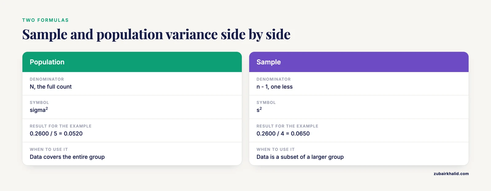
Population variance divides the sum of squared deviations by N, the full count. Sample variance divides by n - 1, one less than the count. Use population variance when your data covers the entire group. Use sample variance when your data is a subset and you want to estimate the wider group.
Why do you divide by n - 1 for sample variance?
Dividing by n - 1 corrects for the fact that a sample is usually less spread out than its population. The sample mean sits closer to the sample values than the population mean does, so dividing by n would understate the true variance. The correction makes the sample variance an unbiased estimator.
Can variance be negative?
No. Every squared deviation is zero or positive, so the sum of squares is never negative. If you get a negative variance, you made an arithmetic or data entry error. Check for a value that was subtracted instead of squared.
How do I find variance on a calculator?
Enter your values into the statistics or list mode, then run the one-variable statistics function. The display shows the sample and population results, often labeled with $s$ and $\sigma$ symbols. The variance is the square of the standard deviation shown, so square the reported value if your model only lists standard deviation.
What does a high variance mean?
A high variance means the values are spread far from the mean. A low variance means they cluster tightly around it. The number is only meaningful next to the scale of the data, so compare it with the mean or with the variance of a similar dataset. For related measures, see the sample variance equation and covariance formula.
References
Further Reading
- 11.2: Introduction to ANOVA's Sum of Squares - Statistics LibreTexts/02%3A_Mean_Differences/11%3A_BG_ANOVA/11.02%3A_Introduction_to_ANOVA's_Sum_of_Squares)
- 12: One-way Analysis of Variance - Statistics LibreTexts/12%3A_One-way_Analysis_of_Variance)
- NIST/SEMATECH e-Handbook of Statistical Methods
- OpenStax. Introductory Statistics 2e
Related Articles
- How to Calculate Variance in Excel (Step by Step)
- Sample Variance Equation: Formula, Steps and Examples
- How to Calculate the Mean: Formula and Step by Step Examples
- How to Calculate Standard Deviation: Formula and Steps
- How to Calculate Midrange: Formula and Examples
- Test Statistic Formula: How to Calculate and Use It