Variance and Standard Deviation Calculators for Lab Data
By Dr. Zubair Khalid, DVM, MS, PhD ·

When a sample variance calculator returns a number that does not match your hand calculation, the most likely cause is the denominator. Many calculators open in population mode, which divides by n, while lab replicates almost always require sample mode, which divides by n-1. The first thing to check is the mode and the count n that the calculator reports. If both are correct, the problem usually sits in the pasted data rather than the math.
This guide explains what variance and standard deviation calculators for lab data actually compute, why their output goes wrong, and how to fix each failure in order from most common to rarest. It closes with a diagnostic sequence, worked examples with realistic assay numbers, and prevention practices that keep results trustworthy.
What a Sample Variance Calculator Computes
Variance describes how far a set of numbers spreads around its mean. It is the average of the squared deviations, where a deviation is the difference between one value and the mean. The standard deviation (SD) is the square root of the variance, which returns the spread to the same units as the measurement. If a plate reader reports absorbance, the SD is in absorbance units and the variance is in squared absorbance units, which is why most people report the SD.
A sample variance calculator assumes your values are a sample drawn from a larger process and computes:
s² = (sum of squared deviations from the mean) / (n - 1)
Here n is the number of values. Dividing by n - 1 is Bessel's correction. It corrects a small underestimate that appears whenever deviations are measured from an estimated mean rather than from the true population mean. Population mode divides by n, and it is correct only when the data include every member of the population you care about, which almost never describes lab replicates.
Two related numbers appear constantly in lab reporting. The standard error of the mean (SEM) equals the sample SD divided by the square root of n, and it describes the precision of the mean rather than the spread of the data. The coefficient of variation (CV) equals the SD divided by the mean, expressed as a percentage. It is unitless, so it compares precision across assays with different scales.
Why Sample Variance Calculator Results Go Wrong
The causes below run from most common to rarest. Each includes the mechanism, because knowing why a number went wrong tells you which fix applies.
1. The Calculator Is in Population Mode
This is the most frequent cause. Population mode divides by n, so the output comes out smaller than the sample value. The relationship is fixed: the sample SD equals the population SD multiplied by the square root of n/(n-1). For n = 5 that factor is about 1.12, and for n = 2 it is 1.41. If the calculator's answer runs consistently below a hand calculation, check the mode first. Spreadsheets expose both versions directly. Excel offers VAR.S and STDEV.S for samples and VAR.P and STDEV.P for populations, and R's var() and sd() always compute the sample versions.
2. Parsing Problems in Pasted Data
Copy-paste carries invisible cargo: tabs, trailing spaces, nonbreaking spaces from PDFs, thousands separators such as 1,234, and decimal commas from other locale settings. A parser may skip such entries, coerce them to text, or read 1,234 as two separate numbers. The symptoms are a variance that changes when you paste the same column twice, or a reported n that does not match your count. The fix is mechanical. Paste through a plain text editor first, put one value per line, strip units and symbols, and confirm the calculator's reported count.
3. Blanks, Zeros, and Censored Values Read as Data
An empty cell pasted as 0, a "not detected" entry, or a value below the detection limit (a censored value) all distort the variance. Zeros inflate the spread and drag the mean down, and a substituted detection limit does the same in the other direction. No calculator can tell which entries are real measurements. Decide the rule before calculating, write it down, and apply it to every dataset the same way.
4. Standard Deviation Confused With Standard Error
Some summary and t-test calculators output the SEM by default. Because SEM = s/√n, a five-replicate dataset shows an SEM less than half the SD. If a figure legend says SD but the calculator supplied SEM, the error bars look tighter than the data warrant. Confirm which quantity the tool returns and label every figure explicitly.
5. Rounding Before the Calculation
Entering values rounded to two decimals when the instrument logged four throws away information. The effect is usually small, but with coarse rounding or few replicates it shifts the variance enough to matter. Keep full instrument precision through the calculation and round only the final reported values.
6. One Outlier From a Failed Well or a Transposed Digit
Variance squares each deviation, so a single bad point dominates. In the worked example below, changing one replicate from 11.8 to 18.1 raises the SD from about 0.51 to about 2.45, a nearly fivefold increase from one digit swap. Sort the values and examine the largest gap before trusting any variance. Verify a suspect point against the instrument record before excluding it, and document the exclusion rule.
7. Systematic Instrument Error That No Denominator Can Fix
A variance calculator assumes the scatter around the mean is random. Systematic error breaks that assumption. Light sources are a classic example. In computer-assisted image analysis of radiographs, an alternating current fluorescent viewbox produced optical density differences tied to light intensity variation, while a direct current halogen viewbox did not [1]. Ultrasound thermometry shows the same hardware sensitivity, because estimates of temperature artifacts depend strongly on the sampling interval and the resolution of the thermometry system [2]. When error is systematic, recalculating in a different tool returns the same wrong answer. Stabilize the instrument and run control materials (reference samples with known values) first, then calculate.
8. Pre-Analytical Processing Differences
Two processing routes through the same protocol can produce different answers from identical samples. In measurements of mitochondrial DNA content in human blood cells, whole blood specimens showed no differences between patient groups, while platelet-depleted mononuclear cell fractions showed group differences of 22% and 40%, because platelets falsify the ratio of mitochondrial to nuclear DNA [3]. The calculator did its job on both datasets. The processing step created the discrepancy.
Safety note: work with human blood and primary cells falls under institutional biosafety procedures, typically Biosafety Level 2, with gloves, eye protection, and surface decontamination after handling.
9. Pseudoreplication and Nested Variance
The deepest cause is the wrong unit of analysis. Technical replicates (repeat measurements of the same sample), biological replicates (independent samples from different subjects or preparations), and separate sessions contribute different variance components, and pooling them treats several measurements of one thing as several independent things. Brain imaging makes the structure explicit. In a task-based functional MRI dataset with 500 trials per subject across 100 scans and 9 to 10 sessions, within-subject variance separated into across-session, across-run, across-block, and residual measurement error components, with measurement error dominant across the whole brain, across-session variance second largest in occipital cortex, and across-run variance second elsewhere [4]. Lab data nest the same way: wells within plates, plates within days, days within operators. Decide what n means before calculating, because the calculator will divide by whatever count it receives.
Troubleshooting Table for Variance and Standard Deviation Calculators
| Symptom | Likely cause | How to confirm | Fix |
|---|---|---|---|
| , - | , - | , - | , - |
| Calculator SD slightly smaller than a hand calculation | Population mode divides by n | Compare the two values, the ratio should match the square root of n/(n-1) | Switch to sample mode and recalculate |
| Reported n does not match your count | Parsing problems in pasted text | Count entries in a plain text editor | Clean to one value per line, remove units and separators |
| Variance changes between identical pastes | Hidden characters or decimal commas | Inspect the raw paste in a text editor | Replace decimal commas, strip thousands separators |
| Error message or a variance of zero | Blanks, text, or censored entries in the column | Scan for "ND", "<", and empty cells | Apply a written rule for censored values, strip units |
| SD far larger than the assay's usual CV | One outlier or a transposed digit | Sort the values, examine the largest gap | Verify against the instrument record before excluding anything |
| Figure error bars look implausibly tight | SEM reported where SD was intended | Divide the SD by the square root of n and compare with the plotted value | Recompute, then label SD or SEM in every legend |
| Two analysts get different variances from one file | Different modes or different rounding | Recompute both ways at full precision | Standardize the template, the mode, and the precision |
| Variance stays high after a clean reanalysis | Systematic instrument error or processing differences | Run duplicates and a control material across the run | Stabilize the instrument or standardize the protocol, then recalculate |
How to Fix a Sample Variance Calculator: A Diagnostic Sequence
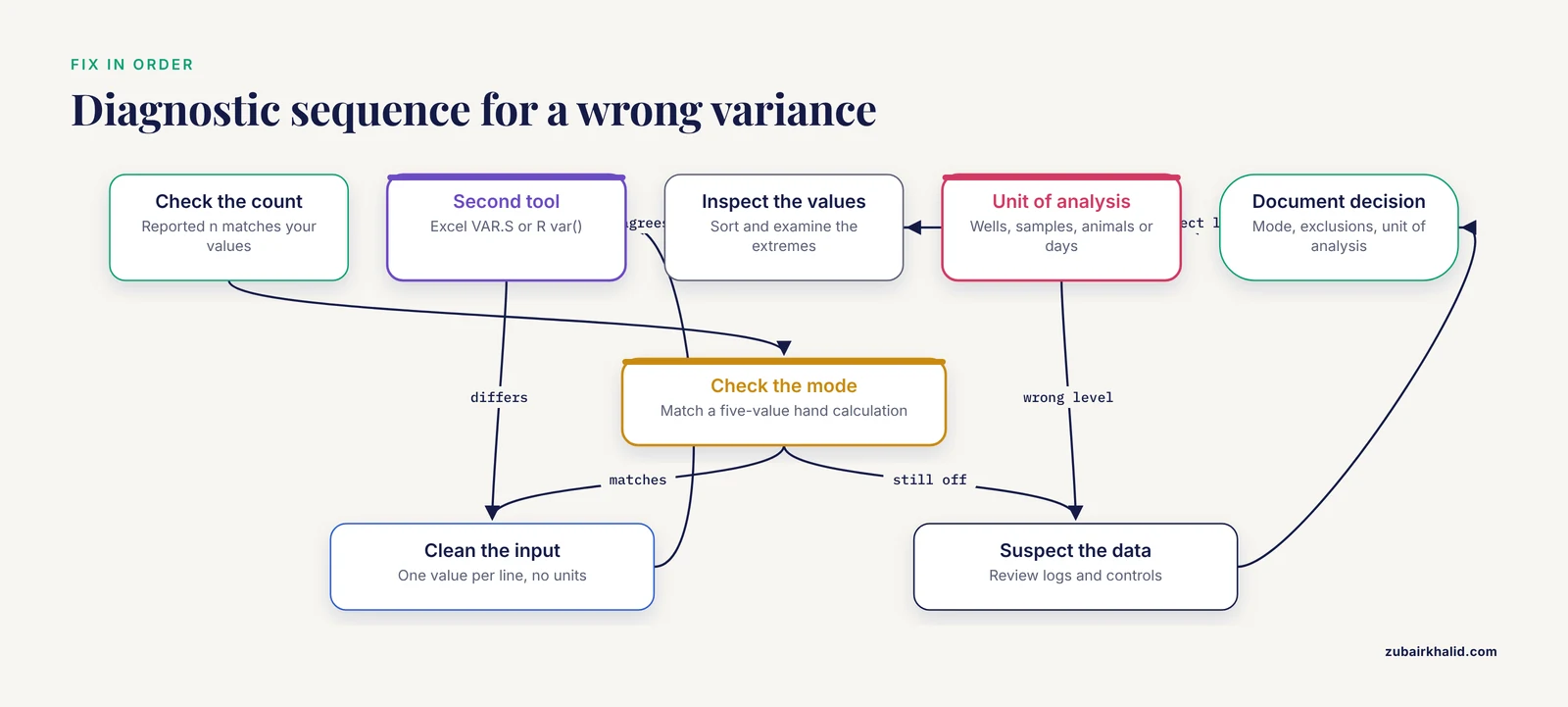
Follow the steps in order. Each one rules out a cause from the list above.
- Check the count. Confirm the calculator's reported n equals the number of values you intended to analyze.
- Check the mode. Run a five-value hand calculation and confirm the output matches the n-1 version.
- Clean the input. Paste through a plain text editor, one value per line, with no units, symbols, or blanks.
- Cross-check with a second tool. Recompute with Excel's VAR.S and STDEV.S or with R's var() and sd(), and require exact agreement.
- Inspect the values. Sort them, examine the extremes, and compare any suspect point against the instrument record.
- Check the unit of analysis. Decide whether n counts wells, independent samples, animals, or days, then recalculate at the correct level.
- Suspect the data, not the tool. If two tools agree and the number still looks wrong, review instrument logs, control records, and processing notes.
- Document the decision. Record the mode, the exclusion rules, and the unit of analysis alongside the result.
Worked Examples With Realistic Lab Numbers
Example 1: Five Replicates of an Enzyme Assay
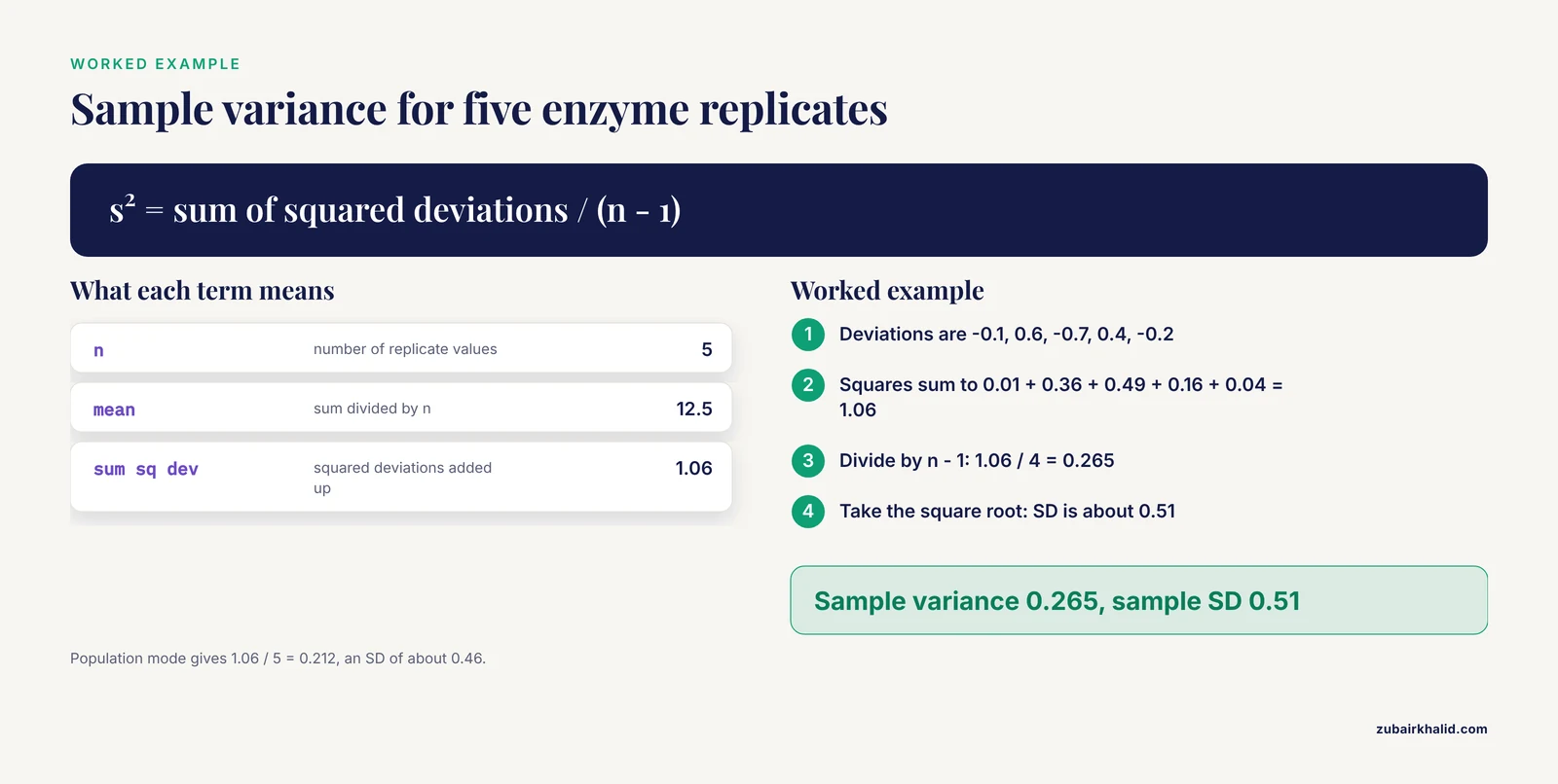
An enzyme assay returns five activity values in micromoles per minute per milligram of protein: 12.4, 13.1, 11.8, 12.9, and 12.3.
The mean is 62.5 divided by 5, or 12.5. The deviations are -0.1, 0.6, -0.7, 0.4, and -0.2, and their squares sum to 0.01 + 0.36 + 0.49 + 0.16 + 0.04 = 1.06.
Sample variance: 1.06 / 4 = 0.265, so the sample SD is √0.265 ≈ 0.51.
Population variance: 1.06 / 5 = 0.212, so the population SD is ≈ 0.46.
The two answers differ by about 12 percent, which is exactly the √(n/(n-1)) factor for n = 5. For lab replicates, report the sample values: 12.5 with an SD of 0.51 micromoles per minute per milligram.
Example 2: SD Versus SEM for the Same Data
The SEM is 0.51 divided by √5, or about 0.23. Writing 12.5 ± 0.51 describes the spread of single assays, while 12.5 ± 0.23 describes the precision of the mean. Both are legitimate summaries, but they answer different questions, and every figure legend should say which one is plotted.
Example 3: Coefficient of Variation Across Assays
The CV for Example 1 is 0.51 / 12.5 × 100, or about 4.1 percent. Because the CV is unitless, it can be compared directly with the CV of an assay measured in different units. Modern materials characterization works the same way. A Bayesian framework for hydrogel mechanical testing quantifies both intra- and inter-sample variability and expresses the coefficient of variation as a function of hydrogel composition, with computational fits within 5 percent error in most cases [5].
From Variance to the Tests You Report
The SD from your calculator is raw material for the tests you report. A quasi-experimental study (one without random assignment) of dental hygiene students' attitudes after interprofessional hospital rotations calculated descriptive statistics and then used independent-samples t-tests and a two-way mixed analysis of variance, which partitions variance across between-subject and within-subject factors, with significance set at p < 0.05 [6]. Each of those procedures consumes a variance estimate, so an error in the upstream SD propagates directly into the test statistic and the p-value.
Sample Size and Power Depend on Your Variance Estimate
Power is the probability that a study detects a real effect of a given size. It rises with the effect size and the sample size and falls as the variance rises. Variance errors are therefore expensive in both directions. Inflated variance inflates the planned sample size, and unrecognized systematic error leaves a properly planned study underpowered in practice.
The light source example above shows the cost in hard numbers. Replacing the alternating current fluorescent viewbox with the direct current halogen viewbox increased design efficiency by 212 percent, meaning the required sample size was 2.12 times greater with the noisy light source [1]. A single instrument choice more than doubled the specimen budget.
Purpose-built design tools encode these relationships. A web-based sample size calculator for nonhuman primate studies, available at midas.wakehealth.edu, covers 11 species and estimates sample counts across longitudinal timepoints while accounting for natural deaths, because power calculations need both a variance estimate and the expected number of animals at each measurement [7].
Rules of thumb lean on the same quantities. For clinical prediction models, classic rules require events per predictor parameter above 10 or 20 and a minimum absolute number of events, and a comparison across 299 published COVID-19 prediction models found that recent formal criteria and these simple rules often agreed on the required sample size [8].
The variance model inside a power calculator matters too. Traditional power calculations rely on restrictive assumptions, and when the variance function is misspecified the output is wrong. Moment-based effect size measures developed for generalized linear models (2SLiP and P2R2) extend to quasi-likelihood settings, where the variance model is specified flexibly rather than through a full distribution, and they remain accurate across diverse outcome types and variance structures [9]. Before trusting a power calculator, check which variance model it assumes.
Variance in Bioinformatics Calculators and Pipelines
Genome-scale data raise the stakes, because effect sizes are small and sample sizes are huge, so even small systematic or random error can create spurious results or hide real ones. Genome-wide association studies therefore run structured quality control in which duplicate concordance infers marker quality and combined analyses of probe intensities and called genotypes flag sample problems [10]. Those QC metrics are variance and agreement calculations running at scale, and a bioinformatics calculator that skips them produces confident nonsense.
Variance estimates also do direct work in effect estimation. Two-sample Mendelian randomization pipelines, which use genetic variants to test whether an exposure influences a disease outcome, commonly apply inverse variance weighting, in which each estimate contributes in proportion to the inverse of its variance, alongside sensitivity methods such as MR-Egger and the weighted median [11]. If the input variances are wrong, the weighted answer is wrong in a way no downstream method detects.
Common Mistakes and Limitations
- Unlabeled error bars. Every legend should state whether bars show SD, SEM, or a confidence interval, because readers cannot tell them apart by appearance.
- Averaging standard deviations across groups. Direct averaging is not a valid combination. With equal group sizes, average the variances and take the square root, or use the pooled variance formula (a sample-size-weighted average of group variances) for unequal sizes.
- Counting technical replicates as n. Three wells from one blood draw are one biological observation with technical replication. The well-to-well variance describes the assay, not the population.
- Calculating variance on pre-summarized data. Feeding group means into a variance calculator discards within-group spread and answers a different question from the one asked.
- Trusting a standard deviation built from three values. With very small n, the SD estimate itself is unstable and its confidence interval is wide. Treat such SDs as rough guides and say so in the text.
- Substituting values for censored data. Replacing below-detection values with zero or with the detection limit distorts the mean and the variance, and the distortion grows with the number of censored points.
- Expecting the calculator to detect bias. A variance calculator assumes random scatter. It cannot see a drifting instrument, a contaminated reagent lot, or a processing artifact.
- Individual datasets vary in structure. For complex designs, repeated-measures structures, or publication-critical numbers, review the analysis plan with a statistician before data collection begins.
Prevention: Sample Variance Calculator Solutions That Last
The durable sample variance calculator solutions are procedural, not mathematical.
- Lock the template. Build a spreadsheet or script with the sample mode fixed, documented, and protected from edits, so the mode question never resurfaces.
- Standardize the handoff. Move data as plain text, one value per line, with units in a header row instead of inside the values.
- Keep full precision. Carry instrument precision through the calculation and round only at the reporting step.
- Run duplicates and controls. Include duplicate samples and a control material in every run, and track their CV from run to run on a simple plot. A rising CV flags instrument drift before it contaminates a dataset.
- Write the rules down. Record the unit of analysis, the exclusion criteria, and the censored-data policy in the protocol before the first value is collected.
- Verify with a second tool. Make the two-tool cross-check routine rather than an emergency measure.
- Date and version everything. A variance number without a date, a mode, and a documented rule set cannot be defended later.
Frequently Asked Questions
What is the difference between sample and population variance on a calculator?
Sample variance divides the sum of squared deviations by n-1, and population variance divides by n. Use the sample version for lab replicates, because they are a sample from a larger process. Use the population version only for a complete census of every unit you care about.
Why does my calculator disagree with my spreadsheet?
The most common reason is a mode mismatch, with one tool in sample mode and the other in population mode. In Excel, VAR.S and STDEV.S are the sample functions while VAR.P and STDEV.P are the population functions, and R's var() and sd() are always sample versions.
Should I use n or n-1 for lab replicates?
Use n-1. Replicates are a sample from a larger process, so the sample formula applies. The n denominator is correct only when the data include the entire population of interest.
What is the coefficient of variation and when should I report it?
The coefficient of variation is the standard deviation divided by the mean, expressed as a percentage. Report it when comparing precision across assays, instruments, or materials with different means or units, because it is unitless.
Why is my standard deviation so much larger than expected?
Sort the values first. A single outlier, a transposed digit, pooled groups, or systematic instrument drift can each inflate the SD severalfold. If the values look clean, the variability may be real and worth reporting rather than fixing.
Can I average the standard deviations from several groups?
No. Direct averaging of standard deviations is not a valid combination. With equal group sizes, average the variances and take the square root, or use the pooled variance formula for unequal sizes.
How many replicates do I need before the standard deviation is trustworthy?
More than two or three. The standard deviation from very small samples is unstable, and its own uncertainty is large. If it will feed a power calculation, collect enough replicates to stabilize it and treat small-sample values as rough guides.
Do I need a special biology calculator for variance work?
No. Any statistics calculator or spreadsheet computes variance correctly once the mode is right. Biology-specific calculators add domain models on top, such as sample size tools for animal studies or quality control pipelines for genomic data, but the core variance math is identical.
Sources
- Light source-induced error in computer-assisted image analysis with a video-based system.
- A two-parameter method for the estimation of ultrasound-induced temperature artifacts.
- Platelets, a typical source of error in real-time PCR quantification of mitochondrial DNA content in human peripheral blood cells.
- Variance decomposition for single-subject task-based fMRI activity estimates across many sessions.
- Non-linear Characterization of Commercial and Decellularized Hydrogels: Statistical Framework Enhanced by Bayesian Optimization.
- Assessing Changes in Attitudes Toward Collaborative Practice Among Dental Hygiene Students: A quasi-experimental study of interprofessional hospital rotations.
- The Non-Human Primate Sample Size Calculator: a design tool for longitudinal research projects.
- Recent criteria and simple rules agreed often on required sample size for developed clinical prediction models.
- Robust power and sample size calculations in quasi-likelihood models: methods and practice.
- Quality control and quality assurance in genotypic data for genome-wide association studies.
- Associations between fatty acids and female reproductive disease risk: A two-sample Mendelian randomization study.