How to Calculate GPA in Excel (Step by Step)

By Dr. Zubair Khalid, DVM, MS, PhD · 2026-10-03

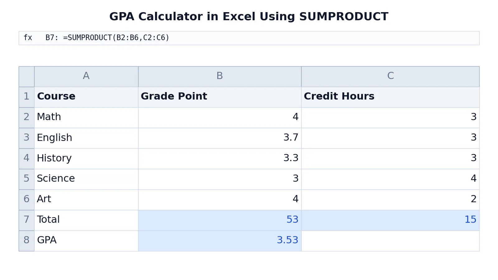
To calculate GPA in Excel, multiply each course's grade point by its credit hours, add those products, then divide by the total credit hours. The SUMPRODUCT function does the multiplication and addition in one step, so a single formula gives you the weighted average. This article shows how to calculate GPA in Excel from a blank sheet, with a worked example you can copy.

Quick Answer

Put grade points in one column and credit hours in the next.
Total quality points: =SUMPRODUCT(B2:B6,C2:C6).
Total credit hours: =SUM(C2:C6).
GPA: =SUMPRODUCT(B2:B6,C2:C6)/SUM(C2:C6).
The result is a weighted average, so a 4-credit course moves your GPA more than a 2-credit course.

Before You Start

You need two numbers for every course. The first is the grade point, the numeric value your school assigns to a letter grade. A common scale is A = 4.0, B = 3.0, C = 2.0, D = 1.0, F = 0. Many schools use plus and minus steps such as A- = 3.7 or B+ = 3.3. Use the scale your own institution publishes, because scales differ.

The second number is the credit hours, sometimes called units or credits. A course worth 3 credits counts three times as much as a 1-credit course.

Set up three columns. Column A holds the course name, column B holds the grade point, and column C holds the credit hours. Keep one row per course and leave no blank rows inside the range. Blank cells are treated as zero by SUMPRODUCT, which quietly lowers your total.

If you are new to writing formulas, the mechanics here are the same as any other Excel formula. See how to make a formula in Excel for the basics of cell references and operators.

Step by Step

Enter your course data. Type the course name in column A, the grade point in column B, and the credit hours in column C. Start at row 2 so row 1 can hold headers.

Label the header row. Put "Course" in A1, "Grade Point" in B1, and "Credit Hours" in C1.

Add a total row. In the row below your last course, type "Total" in column A.

Calculate total quality points. In the total row of column B, enter =SUMPRODUCT(B2:B6,C2:C6). Quality points are grade points multiplied by credit hours, summed across all courses.

Calculate total credit hours. In the total row of column C, enter =SUM(C2:C6).

Calculate GPA. In the row below, type "GPA" in column A and enter =SUMPRODUCT(B2:B6,C2:C6)/SUM(C2:C6) in column B.

Format the GPA cell. Select the GPA cell and set the number format to two decimal places so it reads like a transcript value.

Check the result. Confirm that the total quality points divided by the total credit hours equals the GPA shown.

The formula works because a weighted average is a sum of value-times-weight divided by the sum of weights. Microsoft documents this exact pattern for a weighted average, using =SUMPRODUCT(B2:B7,C2:C7)/SUM(C2:C7) to divide total cost by total units [1].

Worked Example

This is a five-course grade sheet for one semester, with grade points on a 4.0 scale and credit hours per course.

Row	A	B	C
1	Course	Grade Point	Credit Hours
2	Math	4	3
3	English	3.7	3
4	History	3.3	3
5	Science	3	4
6	Art	4	2
7	Total	`=SUMPRODUCT(B2:B6,C2:C6)` -> displays 53	`=SUM(C2:C6)` -> displays 15
8	GPA	`=SUMPRODUCT(B2:B6,C2:C6)/SUM(C2:C6)` -> displays 3.53

The three steps behind those cells:

Multiply each grade point by its credit hours and sum the products. Math gives 12, English 11.1, History 9.9, Science 12, and Art 8. The total is 53 quality points.
Sum all credit hours. The five courses add up to 15 credits.
Divide total quality points by total credit hours. 53 divided by 15 is 3.53.

$$GPA = \frac{\sum (grade\ point \times credit\ hours)}{\sum credit\ hours} = \frac{53}{15} = 3.53$$

Notice that Art has the highest grade point, 4.0, but contributes only 8 quality points because it is worth 2 credits. Science has a lower grade point, 3.0, yet contributes 12 quality points because it is worth 4 credits. That difference is why a simple average of the grade points would give the wrong answer. The plain average of 4, 3.7, 3.3, 3, and 4 is 3.6, which is higher than the true GPA of 3.53.

Other Ways to Do It

Use a helper column. Add a column D for quality points with =B2*C2 in each row, then sum column D and divide by the sum of column C. This is easier to audit because you can see each course's contribution. It is the better choice when you need to explain the math to someone else.

Use AVERAGE with weights. Excel's AVERAGE function ignores weights entirely, so it only matches your GPA when every course carries the same credit hours. Microsoft's guidance on averages covers simple, weighted, and filtered averages, and the weighted case is the one that applies to GPA [1].

Use the GPA calculator tool. If you just want a number and not a spreadsheet, the College & High School GPA Calculator takes your courses and credits and returns the weighted result.

Track a cumulative GPA. Keep one row per semester with semester GPA and semester credit hours, then apply the same SUMPRODUCT pattern across semesters. This gives a credit-weighted cumulative GPA instead of an average of semester GPAs.

Troubleshooting

The GPA looks too high. You probably averaged the grade points instead of weighting them. Check that the divisor is the sum of credit hours, not the count of courses.

The GPA looks too low. Look for blank cells in the grade point column. A blank grade point counts as zero in the multiplication, but the course's credit hours still count in the denominator, so the GPA is pulled down.

A course seems to be ignored. One of the cells in the range contains text. SUMPRODUCT treats text entries as zero instead of returning an error, so the course drops out silently. Remove stray labels, dashes, or spaces from the numeric columns.

The result is a date or a strange number. The cell is formatted as a date or as text. Change the format to Number with two decimal places.

The ranges do not line up. Both ranges inside SUMPRODUCT must be the same size. B2:B6 and C2:C6 pair row by row. If one range is longer, Excel returns an error.

Common Mistakes

Averaging grade points directly. A plain average ignores credit hours and overstates or understates your GPA. Fix it by dividing total quality points by total credit hours.
Using the wrong grade scale. Entering 4.0 for an A- when your school uses 3.7 inflates the result. Fix it by checking your registrar's published scale before typing any numbers.
Mismatched range sizes. Writing =SUMPRODUCT(B2:B6,C2:C7) breaks the row-by-row pairing. Fix it by making both ranges cover exactly the same rows.
Leaving blank grade points or credit hours. Empty cells act as zero. A blank grade point drags the GPA down, and a blank credit hour silently drops the course. Fix it by filling every course row or by excluding unfinished courses from the range.
Counting pass/fail courses as graded. Pass/fail credits usually do not enter the GPA numerator. Fix it by leaving those rows out of the formula ranges.
Forgetting repeated courses. Many schools replace the old grade when you retake a course. Fix it by removing the superseded attempt before you total.

Limitations

This method computes a weighted average of the numbers you type in. It cannot know your school's grade scale, its rounding rules, or how it treats repeated courses, transfer credits, and pass/fail work. Two students with identical grades can have different official GPAs because their institutions apply different policies. Treat the spreadsheet result as your own calculation, not as an official transcript value.

The formula also assumes every course in the range counts toward the GPA. If some courses are excluded, you must adjust the ranges by hand. For large course lists, that manual editing is where errors creep in. A helper column makes those exclusions visible and easier to verify.

Frequently Asked Questions

What is the formula to calculate GPA in Excel?

The core formula is =SUMPRODUCT(grade_points, credit_hours)/SUM(credit_hours). Replace the two range arguments with your actual columns, for example =SUMPRODUCT(B2:B6,C2:C6)/SUM(C2:C6). It returns a weighted average on whatever grade point scale you entered.

Why does SUMPRODUCT work for GPA?

SUMPRODUCT multiplies each pair of cells in the two ranges and adds the results, which is exactly the total quality points you need. Dividing by the sum of credit hours turns that total into a weighted average. It replaces a helper column and a separate SUM with one formula.

How do I calculate a cumulative GPA across semesters?

Build a small table with one row per semester, holding semester GPA and semester credit hours. Then apply the same pattern, =SUMPRODUCT(semester_gpa, credit_hours)/SUM(credit_hours), across those semester rows. If you store semester quality points instead, divide their sum by the sum of credit hours. This weights each semester by its credit load.

Can I use letter grades instead of numbers?

Yes, but you need a lookup step first. Put your grade scale in a small two-column table, letters in one column and grade points in the next, then use a lookup function to convert each letter to its numeric value before the GPA formula runs. The GPA math itself is unchanged.

Does Excel have a built-in GPA function?

No. Excel has no GPA function. You build it from SUMPRODUCT and SUM, or from a helper column of quality points. The weighted average pattern Microsoft documents for other weighted calculations is the same one you use here [1].

If you want to check your arithmetic against a second method, the mean calculation guide explains how averages behave when values carry different weights, and the data analysis walkthrough covers building a small sheet you can trust.

References

Calculate an average | Microsoft Support

References

Further Reading
- Broman KW, Woo KH (2018). Data Organization in Spreadsheets. The American Statistician
- Ziemann M, Eren Y, El-Osta A (2016). Gene name errors are widespread in the scientific literature. Genome Biology
- Microsoft Support: Excel help and learning
- McCullough B, Heiser DA (2008). On the accuracy of statistical procedures in Microsoft Excel 2007. Computational Statistics & Data Analysis
- Abeysooriya M, Soria M, Kasu MS et al. (2021). Gene name errors: Lessons not learned. PLOS Computational Biology