How to Calculate Correlation Coefficient in Excel (Step by Step)

By Dr. Zubair Khalid, DVM, MS, PhD · 2026-10-03

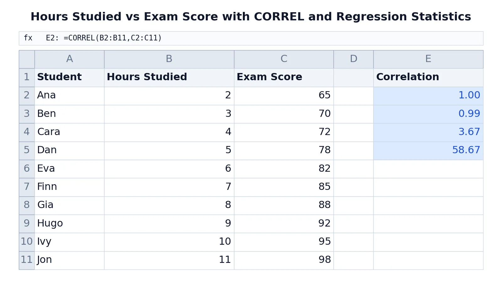
To find the correlation coefficient in Excel, use the CORREL function on two ranges of equal length, or run the Correlation tool in the Data Analysis ToolPak. Both return the Pearson correlation coefficient, a number between -1 and +1 that measures how strongly two variables move together. This guide walks through the formula, the ToolPak route, a full worked example, and the mistakes that produce wrong or misleading answers.

Quick Answer

CORREL takes two ranges and returns the Pearson correlation coefficient: =CORREL(B2:B11,C2:C11).
The result runs from -1 (perfect negative) through 0 (no linear relationship) to +1 (perfect positive) [1].
The Data Analysis ToolPak gives the same number in a correlation matrix, which is handy for three or more variables.
CORREL ignores text, logical values, and empty cells, but it counts cells containing zero [1].
A correlation near 0 means no linear relationship, not that the variables are unrelated in every possible way.

Before You Start

Correlation answers one specific question: how closely do two variables follow a straight line together? It does not tell you which variable causes the other, and it does not capture curved relationships. Keep that in mind before you interpret any output.

Your two ranges must line up row by row. If hours studied sits in B2:B11, the matching exam scores must sit in C2:C11, with each student's pair on the same row. If the ranges have a different number of data points, CORREL returns a #N/A error [1].

You also need variation in both columns. If every value in one range is identical, its standard deviation is zero and CORREL returns a #DIV/0! error [1]. A constant column cannot correlate with anything.

Finally, decide whether you want a single number or a full matrix. For two variables, CORREL is fastest. For three or more, the ToolPak saves time. If you want to check a result by hand or explore the math, the Correlation Coefficient Calculator is a quick cross-check.

Step by Step

Lay out your data in two columns. Put one variable in column B and the other in column C, with a header row. Every row should hold one matched pair of observations.

Pick an empty cell for the result. Click a cell away from your data, such as E2.

Type the CORREL formula. Enter =CORREL(B2:B11,C2:C11) and press Enter. The order of the two ranges does not change the result, so =CORREL(C2:C11,B2:B11) returns the same value.

Read the sign first, then the size. A positive result means the two variables tend to rise together. A negative result means one tends to fall as the other rises. The closer the value sits to +1 or -1, the stronger the linear relationship [1].

Square the result if you want shared variance. The coefficient of determination, or R-squared, tells you the share of variation in one variable explained by the other. In Excel you can get it directly with =RSQ(C2:C11,B2:B11).

For three or more variables, open the ToolPak. Go to Data > Data Analysis > Correlation > OK. Set Input Range to $B$1:$C$11, choose Grouped By: Columns, check Labels in first row, set Output Range to $E$7, and click OK. Excel writes a correlation matrix with 1s on the diagonal.

Label your output. Write "Correlation" or "r" next to the number so the sheet still makes sense weeks later.

The formula CORREL uses is the standard Pearson definition:

$$r = \frac{\sum (x_i - \bar{x})(y_i - \bar{y})}{\sqrt{\sum (x_i - \bar{x})^2 \sum (y_i - \bar{y})^2}}$$

Here $\bar{x}$ and $\bar{y}$ are the sample means, which Excel computes with AVERAGE for each range [1].

Worked Example

Take a small dataset of 10 students, with hours studied in column B and exam score in column C.

Row	A	B	C
1	Student	Hours Studied	Exam Score
2	Ana	2	65
3	Ben	3	70
4	Cara	4	72
5	Dan	5	78
6	Eva	6	82
7	Finn	7	85
8	Gia	8	88
9	Hugo	9	92
10	Ivy	10	95
11	Jon	11	98

Enter these formulas in column E:

Row	E
1	Correlation
2	`=CORREL(B2:B11,C2:C11)` -> displays 1.00
3	`=RSQ(C2:C11,B2:B11)` -> displays 0.99
4	`=SLOPE(C2:C11,B2:B11)` -> displays 3.67
5	`=INTERCEPT(C2:C11,B2:B11)` -> displays 58.67

The correlation is about 0.997 (Excel displays 1.00 at two decimal places), a very strong positive linear relationship. Students who studied more hours tended to score higher. R-squared of about 0.99 means hours studied explains roughly 99% of the variation in scores in this sample.

The slope of 3.67 says each extra hour of study is associated with about 3.67 more points, and the intercept of 58.67 is the predicted score at zero hours. Those two values describe the best-fit line, not the correlation itself, but they are useful context when you report the result.

To get the same correlation through the interface, go to Data > Data Analysis > Correlation > OK, set Input Range to $B$1:$C$11, Grouped By: Columns, check Labels in first row, set Output Range to $E$7, and click OK. The matrix will show 1 on the diagonal and 0.996711 in the lower off-diagonal cell, with the upper triangle left blank.

Other Ways to Do It

The Data Analysis ToolPak is the main alternative to CORREL. It returns a full matrix, so with three variables you see every pairwise correlation at once. That is useful when you screen many columns before building a model.

You can also compute the coefficient manually from the formula above using AVERAGE, SUMPRODUCT, and SQRT. This is slower and easier to get wrong, but it helps you see what CORREL is doing under the hood. If you are building up your spreadsheet skills, our guide on how to calculate the mean in Excel covers the AVERAGE step, and how to calculate standard deviation in Excel covers the spread that feeds the denominator.

For a broader workflow, see how to analyse data in Excel step by step, which puts correlation in context with other summary statistics. If you want the underlying concept before the Excel mechanics, read how to calculate the correlation coefficient step by step.

Troubleshooting

#N/A error. The two ranges have a different number of data points. Check that both start and end on the same rows [1].

#DIV/0! error. One range is empty or has a standard deviation of zero, meaning every value is the same [1].

The number looks wrong. Confirm the ranges are paired correctly. A common slip is selecting B2:B11 against C3:C12, which shifts every pair by one row.

Text or blanks in the range. CORREL ignores text, logical values, and empty cells, but it still counts zeros [1]. If your blanks should be zeros, fill them in before running the formula.

ToolPak missing from the Data tab. The Data Analysis command may not be enabled. Check your Excel add-ins settings and turn on the Analysis ToolPak.

Common Mistakes

Reading correlation as causation. A high r does not mean one variable causes the other. Fix: describe the relationship as an association and look for a plausible mechanism before claiming cause.
Ignoring the sign. A value of -0.9 is a strong relationship, not a weak one. Fix: read the sign before judging the size.
Treating r = 0 as "no relationship." A curved relationship can produce a correlation near zero. Fix: plot the data before trusting the number.
Mismatched ranges. Selecting different row counts or offset ranges breaks the pairing. Fix: build both ranges with the same start and end row.
Leaving outliers unchecked. One extreme point can pull r sharply up or down. Fix: scatter-plot the data and check whether a single point drives the result.
Comparing r across different ranges. A correlation of 0.8 on a narrow range of values is not the same as 0.8 on a wide one. Fix: report the range of the data alongside r.

Limitations

Correlation only measures linear association. Two variables can be tightly linked in a curve, a U-shape, or a threshold pattern and still return a correlation near zero. Always plot the data before you trust the number.

The coefficient is also sensitive to outliers and to the range of values you sample. Restricting the data to a narrow band can shrink or inflate r, and a single extreme observation can move it a lot. Correlation says nothing about causation, and it says nothing about the size of the effect in practical terms. A correlation of 0.99 between hours studied and exam score in a 10-student sample is a strong signal, but it is not proof that more study time alone produces higher scores.

Frequently Asked Questions

How do you calculate the correlation coefficient in Excel?

Use =CORREL(range1,range2) with two ranges of equal length. Excel returns the Pearson correlation coefficient between -1 and +1. For several variables at once, use Data > Data Analysis > Correlation instead.

What is the difference between CORREL and the Data Analysis ToolPak?

CORREL returns a single number for two ranges. The ToolPak returns a full correlation matrix for two or more variables, which is faster when you are screening many columns. Both compute the same Pearson coefficient.

Can the correlation coefficient be negative in Excel?

Yes. A negative result means the two variables tend to move in opposite directions. A value of -1 is a perfect negative linear relationship, and values near -1 indicate a strong one [1].

Why does CORREL return a #DIV/0! error?

CORREL returns #DIV/0! when either range is empty or when the standard deviation of one range is zero, meaning all its values are identical [1]. Add variation to the data or check that you selected the right cells.

Does correlation in Excel prove causation?

No. Correlation measures how closely two variables move together in a straight line. It cannot tell you which variable drives the other, or whether a third factor explains both. Use it as a starting point, then test the relationship properly.

References

CORREL function | Microsoft Support

References

Further Reading
- Broman KW, Woo KH (2018). Data Organization in Spreadsheets. The American Statistician
- Ziemann M, Eren Y, El-Osta A (2016). Gene name errors are widespread in the scientific literature. Genome Biology
- Microsoft Support: Excel help and learning
- McCullough B, Heiser DA (2008). On the accuracy of statistical procedures in Microsoft Excel 2007. Computational Statistics & Data Analysis
- Abeysooriya M, Soria M, Kasu MS et al. (2021). Gene name errors: Lessons not learned. PLOS Computational Biology