How to Calculate P Value in Excel (Step by Step)

By Dr. Zubair Khalid, DVM, MS, PhD · 2026-10-03

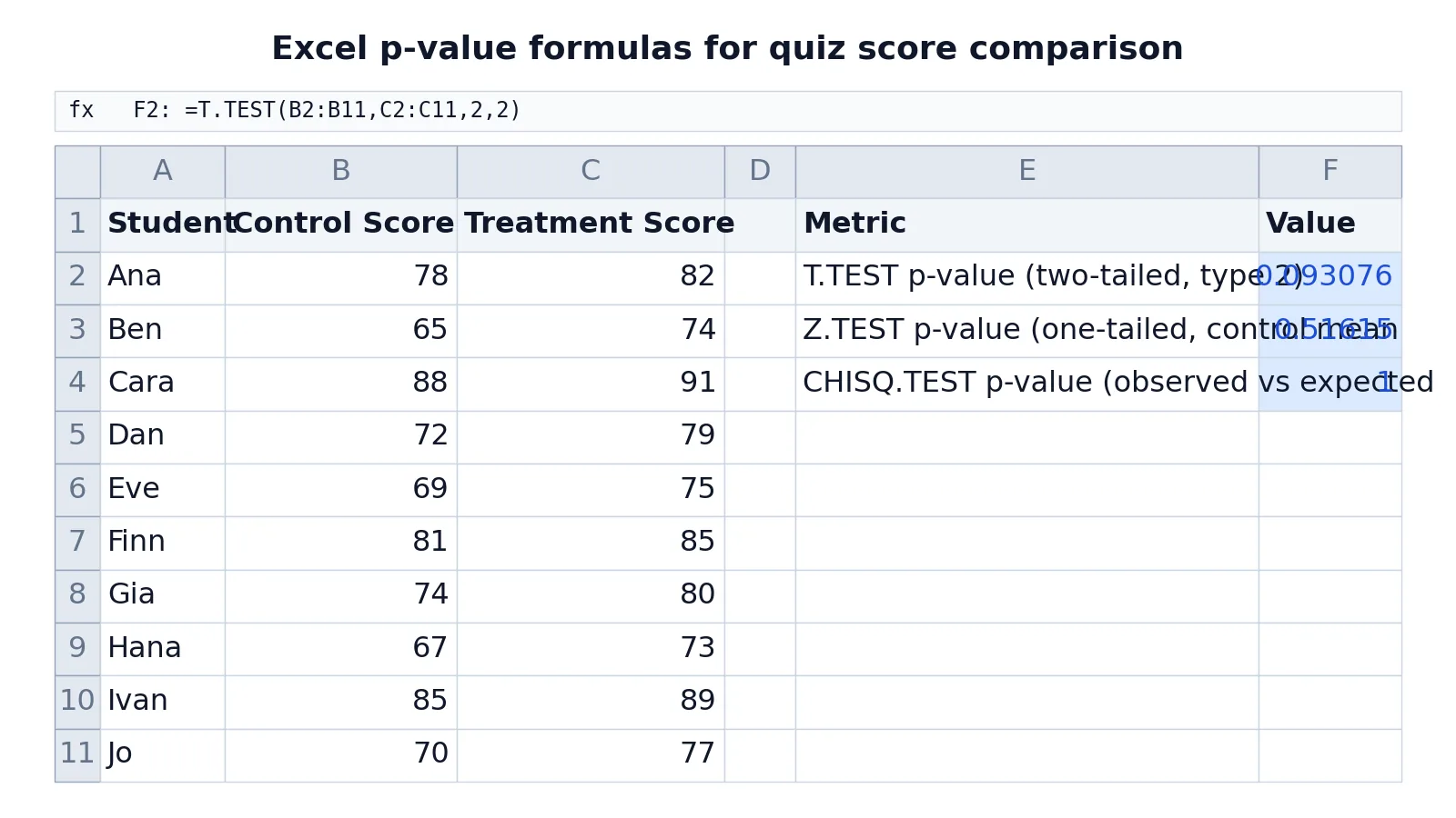
To calculate a p value in Excel you use a built-in test function, not a single arithmetic formula. The function you pick depends on your data: T.TEST for comparing two group means, Z.TEST for one sample against a known mean, and CHISQ.TEST for categorical counts. Each one returns a probability between 0 and 1, and that number is your p-value.

Quick Answer

Two group means, small samples: =T.TEST(array1, array2, tails, type) [1].
One sample against a hypothesized mean: =Z.TEST(array, x).
Observed versus expected counts: =CHISQ.TEST(actual_range, expected_range).
The tails argument is 1 or 2, and type is 1 (paired), 2 (equal variance), or 3 (unequal variance).
A smaller p-value means the observed result is less likely under the null hypothesis [2].

Before You Start

Excel's p-value functions assume your data is already arranged in ranges. You do not type raw numbers into the formula unless you use an array constant. Put each group in its own column or row, with one measurement per cell and no blank cells inside the range.

You also need to decide three things before you write the formula.

First, what is your null hypothesis? For a t-test it is usually "the two group means are equal." For a z-test it is "the sample mean equals a specified value." For a chi-square test it is "the observed counts match the expected counts" [3].

Second, how many tails? A two-tailed test asks whether the means differ in either direction. A one-tailed test asks whether one is specifically larger or smaller. Most exploratory work uses two tails [1].

Third, which test type? For T.TEST, type 1 is a paired test (same subjects measured twice), type 2 assumes equal variances, and type 3 assumes unequal variances. If you are unsure about variances, type 3 is the safer default.

If you need to build the ranges themselves, start with the basics of how to make a formula in Excel and how to sum a column to check your totals before testing.

Step by Step

Enter your data in two columns. Put group 1 in one column and group 2 in the next, with a header row. Keep the ranges the same length for a paired test.

Click an empty cell where you want the p-value to appear.

Type the function name and open parenthesis. For two groups, type =T.TEST(.

Select the first range. Drag over the first group's cells, or type the range like B2:B11.

Type a comma and select the second range. For example C2:C11.

Enter the tails argument. Type 2 for a two-tailed test or 1 for one-tailed.

Enter the type argument. Type 1, 2, or 3 depending on paired, equal variance, or unequal variance.

Close the parenthesis and press Enter. The cell shows the p-value as a decimal.

Format the cell to show more decimals if the value looks like 0. For Z.TEST, the syntax is =Z.TEST(array, x) where x is the hypothesized mean. For CHISQ.TEST, the syntax is =CHISQ.TEST(actual_range, expected_range).

If you want to skip the spreadsheet entirely, the P-Value Calculator returns the same probability from summary inputs.

Worked Example

The dataset below holds quiz scores for ten students under a control condition and a treatment condition. Columns B and C hold the scores, and column F holds three p-value formulas.

Row	A	B	C	E	F
1	Student	Control Score	Treatment Score	Metric	Value
2	Ana	78	82	T.TEST p-value (two-tailed, type 2)	`=T.TEST(B2:B11,C2:C11,2,2)` -> displays 0.093076
3	Ben	65	74	Z.TEST p-value (one-tailed, control mean 75)	`=Z.TEST(B2:B11,75)` -> displays 0.51615
4	Cara	88	91	CHISQ.TEST p-value (observed vs expected)	`=CHISQ.TEST(B2:C11,{78,82;65,74;88,91;72,79;69,75;81,85;74,80;67,73;85,89;70,77})` -> displays 1
5	Dan	72	79
6	Eve	69	75
7	Finn	81	85
8	Gia	74	80
9	Hana	67	73
10	Ivan	85	89
11	Jo	70	77

F2 returns the two-tailed p-value for a two-sample t-test assuming equal variances (type 2) comparing control and treatment scores. The result is 0.093076.

F3 returns the one-tailed p-value for a z-test of the control scores against a hypothesized population mean of 75. The result is 0.51615.

F4 returns the p-value for a chi-square test comparing observed scores in B2:C11 to the expected scores given as an array constant. The result is 1.

Read the t-test result first. A p-value of 0.093076 is above the common 0.05 threshold, so you would not reject the null hypothesis of equal means at that level. The z-test p-value of 0.51615 is far above 0.05, so the control mean is consistent with a population mean of 75. The chi-square p-value of 1 means the observed and expected arrays are identical, so there is no evidence of a difference.

For background on what these probabilities mean, see P-Value Formula and Interpretation: A Researcher's Guide.

Other Ways to Do It

Data Analysis ToolPak. Excel's Analysis ToolPak add-in includes t-Test and z-Test options that output a full table with the p-value included. It has no chi-square test tool, so use CHISQ.TEST for that. You enable it from the Add-ins dialog, then run it from the Data tab. The output gives you more than the single function does, including means and variances.

Manual t statistic. You can compute the t statistic yourself and convert it with =T.DIST.2T(t, df) for a two-tailed p-value. This is useful when you already have a t value from another source. The formula for the two-sample t statistic is:

$$t = \frac{\bar{x}_1 - \bar{x}_2}{\sqrt{s_p^2 \left(\frac{1}{n_1} + \frac{1}{n_2}\right)}}$$

where $s_p^2$ is the pooled variance. This route takes more steps and more chances to make an error, so prefer T.TEST unless you need the intermediate values.

Descriptive checks first. Before testing, confirm your group sizes and centers. The articles on how to calculate the mean in Excel and how to calculate the median in Excel help you spot outliers that would distort a t-test.

Troubleshooting

The result is #NUM!. The tails argument is something other than 1 or 2, or the type argument is something other than 1, 2, or 3. Check both arguments.

The result is #VALUE!. The tails or type argument is not a number. Text cells inside the data ranges are ignored rather than causing an error, so also confirm every cell you meant to include is numeric.

The result is #N/A. The two ranges have different sizes in a test that requires matching pairs.

The p-value looks like 0. Format the cell to show more decimal places. Very small p-values display as 0 until you widen the format.

The result is exactly 1. Your observed and expected arrays are identical, as in the worked example. That is a valid result, not an error.

T.TEST gives a different answer than you expected. Check the type argument. Type 2 and type 3 can give noticeably different p-values when group variances differ.

Common Mistakes

Using the wrong tails argument. A one-tailed test returns roughly half the two-tailed p-value. Decide the direction before you look at the data, and use 2 unless you have a directional hypothesis [1].
Mixing up type 1, 2, and 3. Type 1 is for paired data only. Using it on independent groups gives a p-value for the wrong design.
Leaving blank cells inside a range. Excel treats blanks inconsistently across these functions. Delete empty rows or select contiguous cells only.
Comparing p-values across tests with different assumptions. A t-test, z-test, and chi-square test answer different questions. Do not treat them as interchangeable.
Reporting the p-value without the test details. Always state the test, the tails, and the sample size alongside the number [2].
Treating 0.05 as a hard cutoff. A p-value of 0.049 and 0.051 are practically the same evidence. The threshold is a convention, not a law [3].

Limitations

These functions give you a p-value, not a measure of effect size. A tiny p-value can come from a trivial difference in a large sample, and a large p-value can hide a meaningful difference in a small one [2]. Always report the group means and the sample size next to the p-value.

Excel's p-value functions also assume the data meets the test's conditions. The t-test assumes roughly normal data or large samples. The chi-square test assumes expected counts are large enough in each cell. If those conditions fail, the p-value is not trustworthy, and Excel will not warn you [3].

Frequently Asked Questions

Which Excel function should I use for a p-value?

Use T.TEST when you compare the means of two groups. Use Z.TEST when you compare one sample mean to a known or hypothesized value. Use CHISQ.TEST when you compare observed counts to expected counts. The right choice depends on your data type and your null hypothesis.

What do the tails and type arguments mean in T.TEST?

The tails argument is 1 for a one-tailed test or 2 for a two-tailed test. The type argument is 1 for paired samples, 2 for two samples with equal variances, and 3 for two samples with unequal variances. Both arguments are required.

Why does my p-value show as 0 in Excel?

The true value is smaller than the cell's display precision. Increase the number of decimal places in the cell format, or wrap the formula in a function that shows more digits. The underlying value is still stored correctly.

Can I calculate a p-value without the Data Analysis ToolPak?

Yes. T.TEST, Z.TEST, and CHISQ.TEST are built-in worksheet functions and do not require any add-in. The ToolPak only adds a menu-driven interface and extra output tables.

Is a p-value of 0.05 always significant?

No. The 0.05 threshold is a convention, and whether a result matters depends on context, effect size, and study design [3]. Report the exact p-value and let readers judge it against the standard in your field.

References

- Krzywinski M, Altman N (2013). Significance, P values and t-tests. Nature Methods
- Altman N, Krzywinski M (2017). Interpreting P values. Nature Methods
- Altman N, Krzywinski M (2017). P values and the search for significance. Nature Methods
Further Reading
- Broman KW, Woo KH (2018). Data Organization in Spreadsheets. The American Statistician
- Ziemann M, Eren Y, El-Osta A (2016). Gene name errors are widespread in the scientific literature. Genome Biology
- Microsoft Support: Excel help and learning