How to Calculate the Correlation Coefficient (Step by Step)

By Dr. Zubair Khalid, DVM, MS, PhD · 2026-10-03

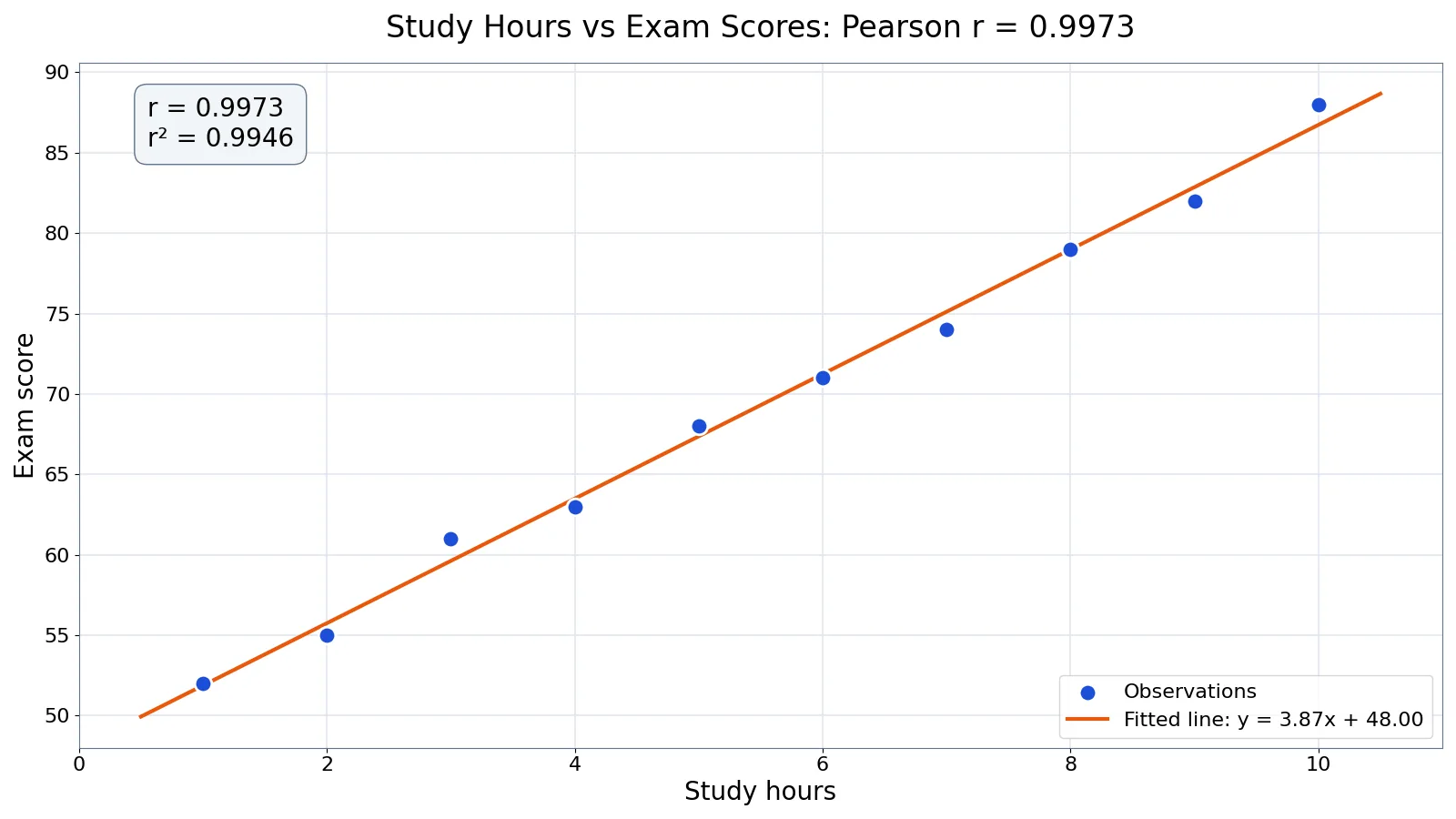
To calculate the correlation coefficient, you standardize each variable, multiply the paired z-scores, and average those products. That single number, Pearson's $r$, tells you the direction and strength of a straight-line relationship between two quantitative variables. This guide shows how to calculate the correlation coefficient by hand, then checks the result in Excel and Python.

Quick Answer

Pearson's $r$ is the average product of paired z-scores, so it always falls between $-1$ and $+1$ [1].
The computational form is $r = \dfrac{\sum (x_i-\bar{x})(y_i-\bar{y})}{\sqrt{\sum (x_i-\bar{x})^2 \sum (y_i-\bar{y})^2}}$.
Sign tells direction. A positive $r$ means high values of $x$ pair with high values of $y$ [2].
Magnitude tells strength. Values near $\pm 1$ mean a strong linear association, values near 0 mean a weak one [2].
$r$ does not change if you switch the two variables or change their units [2].

Before You Start

You need paired data. Each observation must have an $x$ value and a $y$ value measured on the same subject, and the pairs must stay matched. If you shuffle one column, the correlation collapses toward zero.

Both variables should be quantitative. Pearson's $r$ measures a linear relationship, so it is the wrong tool for categorical labels or for curved patterns.

You also need to know which standard deviation you are using. The formula below uses the sample standard deviation with $n-1$ in the denominator, which is the default in most statistics courses and software.

Two quantities drive the whole calculation:

$\sum (x_i-\bar{x})^2$, the sum of squared deviations for $x$.
$\sum (x_i-\bar{x})(y_i-\bar{y})$, the sum of the cross-products.

If you can build those two columns, the rest is arithmetic. The standard deviation guide covers the deviation columns in more detail, and the mean guide covers the averages you subtract.

Step by Step

The formula in z-score form is:

$$r = \frac{1}{n-1}\sum \frac{(x_i-\bar{x})}{s_x}\frac{(y_i-\bar{y})}{s_y}$$

The equivalent raw-score form avoids dividing by the standard deviations first:

$$r = \frac{\sum (x_i-\bar{x})(y_i-\bar{y})}{\sqrt{\sum (x_i-\bar{x})^2 \sum (y_i-\bar{y})^2}}$$

Use the raw-score form for hand calculation. It has fewer rounding steps.

Count your pairs. Call this $n$. Every later step depends on it.
Find the mean of $x$. Add all $x$ values and divide by $n$.
Find the mean of $y$. Add all $y$ values and divide by $n$.
Compute the deviations. For each row, calculate $x_i-\bar{x}$ and $y_i-\bar{y}$.
Square the $x$ deviations and add them. This gives $\sum (x_i-\bar{x})^2$.
Square the $y$ deviations and add them. This gives $\sum (y_i-\bar{y})^2$.
Multiply the deviations row by row and add. This gives $\sum (x_i-\bar{x})(y_i-\bar{y})$.
Divide. Put the cross-product sum on top and the square root of the product of the two squared sums on the bottom.
Check the sign and size. The answer must land between $-1$ and $+1$. Anything outside that range means an arithmetic slip.

Worked Example

Ten students reported their weekly study hours and their exam scores. The table below shows the raw data and the three columns you need.

Hours ($x$)	Score ($y$)	$x-\bar{x}$	$y-\bar{y}$	$(x-\bar{x})^2$	$(y-\bar{y})^2$	$(x-\bar{x})(y-\bar{y})$
1	52	-4.5	-17.3	20.25	299.29	77.85
2	55	-3.5	-14.3	12.25	204.49	50.05
3	61	-2.5	-8.3	6.25	68.89	20.75
4	63	-1.5	-6.3	2.25	39.69	9.45
5	68	-0.5	-1.3	0.25	1.69	0.65
6	71	0.5	1.7	0.25	2.89	0.85
7	74	1.5	4.7	2.25	22.09	7.05
8	79	2.5	9.7	6.25	94.09	24.25
9	82	3.5	12.7	12.25	161.29	44.45
10	88	4.5	18.7	20.25	349.69	84.15

The summary values are:

Quantity	Value
$n$	10
Mean of $x$	5.5000
Mean of $y$	69.3000
Sample SD of $x$	3.0277
Sample SD of $y$	11.7573
$\sum (x_i-\bar{x})^2$	82.5000
$\sum (y_i-\bar{y})^2$	1244.1000
$\sum (x_i-\bar{x})(y_i-\bar{y})$	319.5000

Now substitute into the formula:

$$r = \frac{319.5000}{\sqrt{82.5000 \times 1244.1000}} = \frac{319.5000}{320.3735} = 0.9973$$

The correlation is $0.9973$. Squaring it gives $r^2 = 0.9946$, the coefficient of determination. The regression line fitted to these same points has slope $b_1 = 3.8727$ and intercept $b_0 = 48.0000$.

A value this close to 1 is unusual in real data. It means the ten points sit almost exactly on a straight line, which is what you would expect from a clean teaching dataset.

Other Ways to Do It

Excel. The CORREL function takes two ranges and returns $r$ directly. The Excel correlation guide walks through the function arguments and the Analysis ToolPak route. For this dataset, CORREL returns 0.9973.

Python. NumPy's corrcoef returns a 2 by 2 matrix of correlations. The value at row 0, column 1 is the correlation between the two inputs.

import numpy as np
hours  = [1,2,3,4,5,6,7,8,9,10]
scores = [52,55,61,63,68,71,74,79,82,88]
r = np.corrcoef(hours, scores)[0, 1]
print(r)  # 0.9973

Output:

0.9973

A calculator or an online tool. If you only need the number and not the intermediate columns, the correlation coefficient calculator takes the paired values and returns $r$ and $r^2$. This is the fastest option when you are checking homework or screening a dataset before deeper analysis.

Troubleshooting

Your $r$ is outside $-1$ to $+1$. You almost certainly divided by the wrong quantity or forgot the square root. Recheck step 8.

Your $r$ is near zero but the scatterplot looks curved. Pearson's $r$ only detects straight-line patterns. A perfect U-shape can produce $r$ close to 0.

Your $r$ changes when you reorder the rows. The pairs got separated. Sort both columns together, or use a formula that references matched ranges.

Your hand answer differs from software in the third decimal. Rounding. Keep at least four decimals in the deviation columns, or use the raw-score formula to avoid intermediate division.

One extreme point swings the result. That is a real property of $r$, not a bug. Try the calculation with and without the point to see how much it matters.

Common Mistakes

Mismatching the pairs. If you sort one column and not the other, the correlation is meaningless. Fix: keep the two values for each subject on the same row at all times.
Using the population standard deviation. The formula divides by $n-1$, not $n$. Fix: use the sample standard deviation, which is the default in Excel's STDEV.S and in NumPy's std with ddof=1.
Reading $r = 0.5$ as "half as strong as 1.0." Correlation is not a percentage of a straight line. Fix: judge strength by $r^2$ when you want a proportion, since $r^2$ is the share of variance explained.
Treating correlation as causation. Two variables can move together because a third variable drives both. Fix: describe the association and stop there unless you have a designed experiment.
Ignoring the shape of the scatterplot. A single number hides curves, clusters, and outliers. Fix: always plot the points before you trust $r$.
Dropping missing values inconsistently. If you remove a row for $x$ but keep it for $y$, the pairs no longer line up. Fix: drop the whole row whenever either value is missing.

Limitations

Pearson's $r$ measures linear association only. It cannot detect a strong curved relationship, and it can report a value near zero for data that are perfectly related in a non-linear way. It is also sensitive to outliers, since a single distant point can pull the value substantially in either direction.

The coefficient says nothing about causation, and it says nothing about the size of the effect in the original units. A high $r$ between two variables that both rise over time is often just a shared trend. When you use $r$ to judge how well a regression fits, treat it with care, because $r$ and regression answer different questions and a good fit in one does not guarantee a meaningful result in the other [3].

Frequently Asked Questions

What is the difference between $r$ and $r^2$?

$r$ is the correlation coefficient and runs from $-1$ to $+1$. $r^2$ is the coefficient of determination, always between 0 and 1, and it tells you the proportion of variance in one variable explained by the linear relationship with the other. For this dataset, $r = 0.9973$ and $r^2 = 0.9946$.

Can the correlation coefficient be greater than 1?

No. Pearson's $r$ is bounded between $-1$ and $+1$ [2]. If your calculation returns something like 1.53, you have made an arithmetic error, most often by dividing by the wrong sum or by omitting the square root.

Does it matter which variable I call $x$ and which I call $y$?

No. Switching the roles of the two variables leaves $r$ unchanged, and the same is true if you change the units of either variable [2]. That symmetry is one reason $r$ is easy to report, but it also means $r$ alone cannot tell you which variable influences which.

How many data points do I need?

There is no hard minimum, but small samples give unstable estimates. With fewer than about 10 pairs, a single unusual point can move $r$ a long way. Report $n$ alongside $r$ so readers can judge how much weight to give it.

What does a negative correlation coefficient mean?

A negative $r$ means high values of one variable tend to pair with low values of the other [2]. The strength is judged by the absolute value, so $r = -0.80$ is a stronger linear relationship than $r = 0.60$.

References

4.1: Scatterplots and Correlation - Mathematics LibreTexts
2.3: Correlation - Statistics LibreTexts/02%3A_Bi-variate_Statistics_-_Basics/2.03%3A_New_Page)
Use the Correlation Coefficient to Summarize Regression Performance? - PMC